MY REFERENCE FOR LEARNING
and SOME RESOURCES I’M COLLECTING ALONG THE WAY
Maya’s node based architecture, nodes with attributes that are connected gives Maya its flexible procedural qualities. Each node performs some operation on the data that is passing through it with each node having attributes to accomplish a specific task.
Dynamics is the complex physical mechanism that determines how objects move to simulate real-world forces using the rules of physics. Simulating the complex motion of natural forces in animation and effects by creating an environment with elements that react to the forces applied (fields, expressions, goals etc) creating effects with motion such as fireworks, lightning, shatter, smoke, rain, fire, colliding objects, curve flow, surface flow etc. This includes rigid bodies, soft bodies, particles, dynamic constraints and rendering. Rigid bodies can be active or passive controlling how the bodies collide and react with each other. Active objects typically fall, move, spin and collide with passive objects such as a ball falling to the floor.
Specifying the different actions for the object to take and the software will figure out how to animate that object in the most realistic way by assigning physical characteristics that define how an object behaves in a simulated world.
Special Effects Animations simulate physical phenomena such as collusions, smoke, fog, clouds, water, cloth, fire, explosions, hair, grass, fur and natural movements of colliding bodies creating realistic-looking motion based on the principles of physics. Dynamic animation lets you create realistic motion that’s hard to achieve with traditional keyframe animation.
Objects are converted to dynamic bodies through attributes which affect how they behave and are affected by external forces called fields such as wind and gravity. Dynamic bodes such as particles which are point sin space that have renderable properties, hair consists of curves and fluids are essentially volumetric particles.
PHYSICS CONCEPTS
Newton’s first law:
Force = Mass x Acceleration F = ma
In Dynamics Force and mass are known quantities then acceleration is calculated by the dynamics system based on these values controlling the particle’s motion.
Force coming from things such as fields, springs, expressions and Mass exists by default then a = F/m
ORDER OF EVALUATION
- Acceleration
- Particle Runtime Expressions before Dynamics
- Forces includes fields, springs, goals
- Velocity computed from the acceleration
- Positions computed from velocity
- Runtime Expressions after Dynamics
PARTICLES
Are reference points, points in space with no size or volume, used for special effects such as fire, fireworks, lightening, shatter, curve flow, surface flow, sparks, shockwaves, energy pulses, gases, dust, snow, rain and smoke that can collide with geometry and affect rigid bodies. Particles are displayed, selected, animated and rendered differently, can be seen as collective objects or used with array attributes as individual particles using ramps, scripts and expressions. Particles can be considered to have a collective transform also containing attributes that control individual particles using Array attributes including ramps, scripts and expressions.
Individual particles can be thought of as components to the particleShape node, commonly categorised into two types: Per Particle (array), and Per Object. As they do not contain surface information they require special handling at render time. Particles have Per Particle, often with PP at the end of the attribute (array) which allows each particle to store its own value for a given attribute and Per Object assigns one attribute value to the entire particle object.
- Per Particle: each particle stores its own values
- Per Object Attribute: assigns one attribute value to the entire particle object
Particle objects can be keyframed (translate, scale, rotate) keeping in mind which axis of rotation is being used or controlled dynamically.
Normalised age is the relationship between a particle’s age and its lifespan (age/lifespan).
Vector qualities such as position, acceleration and velocity using a Ramp Editor the RGB corresponds to the particle’s X, Y, Z respectively.
Propagation calculations for the current frame are determined by the previous frame for attribute values.
Values greater than 1 for float attributes with a ramp, open the Colour Chooser window and switch to HSV move, enter the desired value in the V field.
Colour images used as a multiplier with luminance of 0 for black and 1 for 100% emitter’s rate.
Play Every Frame in Settings/Preferences. When opening a scene the time setting will be read from the scene file.
Animating particles though fields, dynamic expressions and the transform (translate, scale and rotation). They can be keyframed or controlled dynamically as a group.
Individual particles cannot be removed, can set particle opacityPP to 0, lifespanPP to 0 using the particleId in an expression or setting the value in the Component Editor.
Individual particles are components of a particleShape object as vertices of geometric objects belong to their shape node.
- Fields such as gravity, turbulence, air, vortex
- Expressions provide mathematical control such as sin and rand
- Collisions are methods for creating and killing particles when they collide with geometry
- Emit creates and positions particles
PARTICLE, EMITTER, RENDER ATTRIBUTES
- Acceleration: a vector, measurement of the change in velocity over time
- Colour Accum: affects overlapping particles and how they get their RGB values added together, ON overlapping particles within the same particle object get their RGB values added together
- Colour
- Conserve: is conservation of momentum, set at 1 the particles never lose their motion, very sensitive attribute
- Current Time the default is the scene time, can create a custom time curve, cached particles can be edited in the Graph
- Density
- Depth Sort: draws the particles from back to front
- Direction: X, Y, Z
- Editor
- Force In World
- Friction controls slipperiness or energy loss, static, dynamic
- geoConnector: inputs attributes of Resilience controls how much rebound occurs, Friction
- Glow Intensity
- Incandescence
- Inherit Factor: controls how much of the emitting objects velocity is transferred to the particles during emission
- Initial State: the values that exist at the initial frame
- Level of Detail
- Lifespan: how long the particles stay in the scene before disappearing, unit is usually seconds fps in the settings. Check if reading from the scene file or the preferences. (Live Forever exists indefinitely, Constant die when the Lifespan is reached which is measured in seconds, Random Range allowing some particles to live longer than others by setting the range, LifespanPP Only used with expressions, Particle Size radius includes being able to randomise the radius size)
- Line Width
- Mass will not affect how the object falls under the force of gravity. Affects how much force is exerted when a collision occurs and how non-gravity fields will move the object.
- Max Count: limits the total number of particles the selected particle object is allowed to hold, -1 means there is no limit on the number of particles
- Min and Max Distance emits particles within an offset distance from the emitter
- Multi Count
- Multi Radius
- Normal Speed: along the vector that is normal to the point of emission, 0 will have no speed, sticking to the surface
- Opacity: the vertical axis represents normalised age, the bottom represents the birth with the top corresponds to its death
- Position
- Radius: black = 0, white = 1
- Radius Scale Input: Normalised Age is the relationship between a particle’s age and its lifespan (age/lifespan). When a particle’s age is equal to its lifespan, the particle dies.
- Rate Particles/Sec: is the number of particles per time unit,
- Render Type: MultiPoint, MultiStreak, Numeric, Points, Spheres, Sprites, Streak, Blobby Surface (s/w), Cloud (s/w), Tube (s/w)
- Resilience: controls how much rebound occurs in the particle collision, can use negative numbers
- Speed: how fast the particles leave the emitter, measurement of rate only without respect to direction
- Speed Random randomises the speed
- Spread: adjusts the cone angle
- Tail Fade and Size
- Tangent Speed: along a randomly selected vector that is tangent to the surface of emission, 0 will have no speed sticking to the surface, moving perpendicular to the faces, increase a little and the particles will move along the surface tangent from which they originate.
- Use Lighting
- Velocity: is a vector, a particle’s change in position over time measured in Rate and Direction
PARTICLE EMITTERS generate moving or stationary particles as an animation, can create smoke, fire, fireworks, rain, and similar objects.
- Directional emits a spray in a specific direction
- Omni equally in all directions, can be emitted from vertices, CVs of objects and curves
- Volume emits from within a specified volume
- Curve from the portions of the curve between the CVs or from points
- Surface direction of the normals
- Per-Point
- Texture
Consider:
- Direction
- Speed: how fast the particles leave the emitter
- Rate: number of particles per time unit
- Spread: 1 = 180 degree emission cone
- Time: default unit is seconds
- Distance/Direction attributes are relative, value of 1 for X and a value of 2 for Y makes the particles spray at twice Y of their distance X
- Tessellation Factor controls the level of detail of the surface that emitters use
PARTICLE SHAPE NODE default attributes:
- Transform node
- Position
- Velocity
- Accelearation
- Mass
PARTICLE SHAPE NODE some attributes that can be added:
- Lifespan
- Radius
- Colour
- Incandescence
- Opacity
COLLISIONS Particles can collide with geometry and not each other, can be caused by either moving particles or by moving or deforming geometry.
Trigger:
- Emit new particles
- Execute a MEL procedure
- Kill particles
PARTICLE COLLISIONS EDITOR choose actions to occur when a particle collides with its collision objects. Emit keeps the particle in the scene resetting the age to 0, Split kills the particle starts the age of the new particle at whatever value the old particle’s age was when the collison occured
- All Collisions
- Collision Number
- Type
- Random # Particles
- Num Particles
- Spread
- Target Particle
- Inherit Velocity
An Event Procedure is typically a MEL script that is called when a collision occurs and the event is triggered. The following format and argument list:
global proc myEventProc (string $particleName, int $particleId, string $objectName)
- $particleName – the name of the particle object
- $particleId – the particle number of the particle that has collided
- $objectName – name of the object that the particle has collided with
closestPoinOnSurface returns information about a point on the surface n relation to the worldspace position information
pointOnSurface is an operation that can create a pontOnSurfaceInfo node
- Resilience
FIELDS: air, drag, gravity, newton, radial, turbulence, uniform, vortex are used to move particles around in the scene.
Gravity is measured in meters per second squared, at the Earth’s surface the acceleration of gravity is about 9.8 metres (32 feet) per second per second. Maya is often in centimetres, not meters, adjust the gravity magnitude. 980 is the correct magnitude when working in centimetres.
FILEDS ATTRIBUTES: note the axis as controlled by the field’s world axis or local which can be controlled by parenting to the particle object. Can consider using a ramp instead of a field and including textures mapped to the ramp.
- Magnitude
- Attenuation controls an exponential relationship between the strength of the field and the distance between the affected objects. 0 causes a constant force regardless of the distance
- Frequency
- Max Distance
- Use Max Distance
- Direction
- Speed
- Component Only
- Spread
INSTANCING: The instance does not contain actual surface information, it is a redraw version of the original object and updating as the original is updated.
Particles can be used to control the position and motion of instanced geometry including instancing a keyframed object to particles, cycling through a sequence of snapshot objects to create the instanced motion or providing an aim control of the instanced object which could be a textured plane that is aimed at the camera.
Custom attributes need to be connected in the pop-up menus of the Instancing (Geometry Replacement) section for the particleShape1 node of the Attribute Editor. Needs to be the same data type, consider enabling Allow All Data Types.
- Aim Direction
- Aim Position
- Aim Axis
- Aim Up Axis
- Aim World Up
- Cycle
- Cycle Step Size: how long the index displays the object before switching to the next item in the list
- Level of Detail
- Object Index
- Position
- Rotation
- Rotation Order
- Rotation Type
- Rotation Units
- Scale
- Shear
- Visibility
Michael Mileski – ARCHIVE FOR THE TAG “SPRITES”
EXPRESSIONS and MEL COMMANDS: An almost limitless method o controlling particle parameters sharing the MEL syntax and methodology. Functions such as linstep(), sin() and rand() provide mathematical control over particle appearance and motion.
- nParticle -name droplets; in the command line, created a particle object named droplets
- particleShape1.mass = 5;
- internalVar -userScriptDir; to find where Maya is looking for scripts
Each particle has its own unique numerical identity – particleId is an integer value ranging from 0 to -1. The first particleId is 0.
The % symbol stands for the modulus operation which is the remainder produced when two numbers are divided.
GOALS: A location in space, a destination point for particles that can be animated including individual particle control, multiple goal objects with per particle attributes and transferring from one particle to another. The goal weight controls the deviation of the soft body from its goal object. Goals can be curves, lattices, polygons, particles and attributes include Goal Weight, Smoothness and Per Particle Goal attributes.
- Goal Smoothness
- targetFocusShape
- Goal Active
Consider:
- Dynamics Weight: 0 will not compute
- Conserve: if particles overshoot the goal
- Level Of Detail
- Inherit Factor: inherited velocity
- Goal Weight
- Goal Smoothness
- MinMax RangeU
- MinMax RangeV
- Growth
SPRINGS: can be applied to any particle and dynamic geometry which includes attributes of softness, rest length and damping for control on a per object or per spring basis.
PARTICLE TOOL: create individual particles, grids and random collections
- Name
- Number of Particles
- Sketch Particles
- Maximum Radius
- Sketch Interval
Relative: receives the transform information from the Transform node directly above it in the hierarchy preventing double transformations when parented to geometry.
DYNAMIC BODIES
Making the surface points dynamic
- Soft: malleable surfaces that deform dynamically such as a fluid-like motion.
- Rigid: solid objects – active which is affected by collisions and fields – passive is not affected by fields
Soft bodies are surfaces that have particle-like control on their CV’s or vertices. Soft bodies connect surface geometry with dynamic bodies, indirectly affect skinned surfaces using dynamic influence objects, modelling, collision modelling and fluid-like effects. Particles do not collide with each other, do not obey interpenetration checking with Unlimited Cloth being an exemption.
The particle object is created and parented under the object. The particle object is placed in relation to the surface, placed on the corresponding CVs or vertices and the surface will follow the particles when the particles are moved the shape of the geometry will change.
Fluid-like motion with geometry that has particles controlling the position and movement. Goals using Goal Weight and Springs using attributes such as Stiffness, Rest Length and Damping are ways of controlling soft bodies.
A duplicate surface can be created and used as a goal object making the original selected object the soft body, the duplicate can be made soft thus making the original the goal object.
Soft bodies provide a direct manipulation of surface geometry with dynamic forces also indirectly affecting skinned surfaces through dynamic influence objects. Some limitations are that the particles do not collide with each other or obey interpenetration checking of the surface.
SPRINGS and soft bodies are often used together as goal objects are not always appropriate for controlling a soft body that is deforming or colliding with another object. Useful for controlling particles responding to forces with cohesion, can be established between particles and CVs or vertices and between surface CVs or vertices. Springs can be created between different soft body objects or between soft body objects and geometry.
When a polygonal object is used as a soft body goal the particles will move towards each of the vertices in turn. Particle 0 to vertex 0 etc.
Consider:
- Wire Walk Length along the wireframe segment
- All between all the selected components
- Max/Min between the selected components that fall between the Min and Max
- Set Exclusive between objects and not between components
- balance between the springs and the force of gravity
- StiffnessPP
- DampingPP
- RestLengthPP
- GoalPP
- End1Weight
- End2Weight
- GoalWeight[0]
- Stiffness
- Damping
- Conserve
- geoConnector – Resilience, Friction
- Oversampling
RIGID BODIES
Provides the animation of geometric objects in a dynamically controlled, collision-based system that are created to collide and react with one another, causing and responding to collisions. Normal orientation of a surface is required for rigid body collisions. Single sided polygonal surfaces will not collide correctly. Extrude the face a little. Can only have one rigid body controlling a given hierarchy.
- Tessellations
- Normals
- StandIns
- Bake
- Collision Layers
- Multiple Solvers
- Scene Scale and Units
ACTIVE vs PASSIVE
Can keyframe active/passive state to combine keyframing and dynamic action together. The state of the rigidSolver can be set to On and Off in the rigidBody node of the Attribute Editor. Consider using the Set Active or Set Passive menu options under the Soft/Rigid Bodies. Ignore may need to be keyframed one frame before anther important operation.
- Impulse: keep moving in a given direction
- Spin Impulse: to spin around the specified axis
- Initial Spin: a force at the first frame to cause spinning around the defined axis
ACTIVE RIGID BODIES
Active objects typically fall, move, spin and collide with passive objects, respond to collisions, cause collisions, are not keyframed and are affected by fields.
- Solver controls the rigid bodies dynamics
- Time controls when the rigid solver’s evaluations take place
MEL command to select the rigidBody only: select ‘ls -typ “rigidBody”‘;
PASSIVE RIGID BODIES
Can be keyframed, cause collisions, do not respond to collisions and are not affected by fields.
Controls the evaluation of the rigid body dynamics, rigid bodies are controlled by the attributes on the rigidSolver node and the time node. Errors can result when values are changing or exceeding the proper expected range thus making assumptions as a trad-off between accuracy and interaction. The position and orientation of all rigid bodies are calculated using rules inside each frame to produce the final result. Objects cannot collide or be influenced by objects on separate solvers.
To move a rigidBody to another solver:
rigidBody -edit -solver -rigidSolver1;
Any object whose surface does not deform when a collision occurs, does not change shape eg metal rod, floors, ceilings, cricket ball. Curves, particles and lattices cannot become rigid bodies as they have no surface information. Surfaces made from these can be rigid bodies. The collision calculations are based on the original, non-deformed object Particle collisions can collide with deforming geometry and deforming rigid bodies.
- Mass is a factor in how much momentum is transferred from one object to another
- Static and Dynamic Friction is how much friction there is at rest and when in motion, how much the object resists moving or being moved, 0 is not friction
- Bounciness is how resilient the body is upon collision
- Damping creates a drag on the object in dynamic motion
- Frictions
- Initial Velocity gives an initial push
- Initial Spin gives an initial twist
- Impulse Position gives a constant push
- Spin Impulse rotates constantly in the desired axis
- Centre of Mass is at the pivot point, the offset the centre of the mass
- Collision Layer
- StandIn
- Active
- Collusions
- Step Size
- Collision Tolerance
- Start Time
- Rigid Solver Method
- Apply Forces At
The rigid body’s performance attribute to the varying speed of simple collisions by telling the solver how to calculate the piece of geometry as a simple primitive. Stand-ins maybe used when the playback is slow reducing the number of vertices, adjusting tessellation values, interpenetration errors, displaying in wireframe, hiding unused objects etc the solver is keeping track of. Avoiding interpenetration errors includes, adjusting the rigidSolver attributes of step size and collision tolerance, increasing damping to avoid wild velocities, checking surface normals and positioning objects with a little gap.
Make the Stand In geometry a rigid body, then parent the higher resolution object to the Stand In and hide the Stand In.
- None calculates each vertex
- Cube
- Sphere
Allow dynamic objects to be constrained or constrain each other.
- Nail: an Active Rigid Body to a point in space which can be grouped and translated under another object as a child
- Barrier: creates a planar boundary that an Active Rigid Body cannot pass through
- Pin: two Active or an Active and Passive Rigid Body to each other, the pinning point or pivot is adjustable and can be keyframed
- Spring: two Active or an Active and Passive Rigid Body to each other or a point in space
- Hinge: two Active or an Active and Passive Rigid Body with a user defined pivot orientation, constrained to one axis and also to a point in space
- Directional Hinge: the difference is that the orientation of the hinge axis will change depending on the motion of the object(s) that it is connected to.
- Slider
- Point
- Cone-Twist
- 6 Degrees of Freedom
- Spring 6 Degrees-of-Freedom
DYNAMIC CONSTRAINTS ATTRIBUTES
The mass of all rigid body pieces directly affects the motion of the simulation. Individual values can be found in the Attribute Spread Sheet.
Half the original value in the Channel Box type: /=2
Objects on the same collision layer number will collide with each other, different numbers will not. An object on layer -1 will collide with any collision layer. It is clearly visible to see which objects will be colliding by looking at the Attribute Spread Sheet.
Set Rigid Body Interpenetration and Set Rigid Body Collisions under Solvers menu produces the same basic result as setting different objects on different collision layers.
Will save the current pose as the Initial State, retaining this shape or pose for the beginning of the sequence. Not necessarily the first frame in the playback range, determined by the Start Frame attribute on each particle object.
Converting one type of action or procedure into another, baking dynamics into keyframes. After baking the simulation Rigid Bodies, Rigid Constraints and Static Channels can be deleted.
Through the graph editor retaining the curve’s basic shape and losing some of the unneeded keyframes.
Particles following a shape such as a curve eg a tornado or surface eg lava. Deformers using clusters can be added to curves and including fields.
Shape Keyable Tab
nPARTICLES
Newton’s first law – Force = Mass x Acceleration, F = ma – a = F/m
Particles are moved dynamically using collisions and fields, often used as larger systems used together to create an effect with dynamic attributes for the motion of the system as a whole. A Particle is a point in space with renderable properties which can create effects such as smoke, fireworks, steam etc.
- Shading > Colour Ramp
- Opacity > Scale Ramp
- Radius > Radius Scale
PARTICLE INSTANCING: to control the position and motion of instanced geometry such as a keyframed object to a particle.
COLLISIONS
- Emit keeps the particles in the scene, resetting the age of the new particle to 0
- Split kills the particles, starts the age of the new particle at whatever value the old particle’s age was when the collision occurred
EXPRESSIONS are instructions given to Maya that control attributes over time, they are evaluated in the order they appear in the Expression Editor. Expressions can provide solutions for getting results that would be difficult or impossible to keyframe.
- Scaler: numerical quantity with one specific component eg time, mass
- Vector/Position: quantity with magnitude and direction, location <<1, 2,3>>
- Float: decimal numerical value
- Integer: non-decimal whole number
- String: collection of alphanumeric characters
- Boolean: value either true or false, on or off, 1 or 0
- Variable: location in memory used to store data information
- Propagation: calculate the values based on the result from the previous frame
- Creation Expression: evaluated only once for each particle in the particle object when the particle is born, stored in the creation portion of the Expression Editor for that particle
- Runtime Expression: before Dynamics, after dynamics, evaluated at least once per particle per frame but not at birth, stored in the runtime segment of the particle object in Expression Editor
- Linstep: linear curve
- Smoothstep: linear curve with an ease-in and ease-out
Individual particles cannot be removed though can use opacityPP = 0
mag function is used to find the magnitude of a vector, also know as the length, distance
Initial State attribute is designated by the 0 as in position0, velocity, acceleration mass etc
A BEGINNER’S INTRODUCTION TO MAYA EXPRESSIONS
An object that particles follow or move towards controlling particle position and motion. Goals can be created from curves, lattices, polygons, NURBS surfaces, particles or transform nodes and can include multiple goal objects.
- Goal weights are set on a per particle basis controlled by the goalPP attribute. When more than one object is an active goal the resulting total will be a combination of the goal objects’ positions and the Goal Weights that are set for each goal on the particleShape. A goal weight of 1 means the particle will stick to its goal immediately, 0 it will not move towards the goal. The goalPP weight is multiplied by the Goal Weight of the particle object for a total particle weight. When a value is 0 and the goalPP is 0.5 the resulting goalPP value will be 0, not 0.5 as would be expected.
- Goal Smoothness is how the particles accelerate towards a goal object. Low value the particles take large steps, high value smaller steps.
- Goal Active goal object’s influence On and Off
- Dynamics Weight how much the various dynamic contributors such as fields, affect the particle object, 0 has no effect
- Conserve controlling the acceleration of particles in particular if the particles overshoot
- Inherit Factor controls the amount of velocity inherited from the emitting object when an object’s animation is involved
- Emissions in World emission are in world space
- GoalUV
- Min Max Range U and V
The ratio between Goal Smoothness and Goal Weight controls how far the particle will travel towards the goal in each step.
Use display layers to hide goal objects.
Need Parent UV
Set nParticle attributes using expressions or MEL
COMMON TERMS
- Scalar: a numerical quantity with only one specific component eg Time and Mass
- Vector: has magnitude and direction represented as three distinct numerical components eg <<1,2,3>>
- Float: decimal numerical value eg 1.2
- Integer: non-decimal whole number eg -1, 10
- String: collection of alphanumeric characters eg “street463”
- Boolean: ture or false value, on or off, 1 or 0
- Variable: location in memory used to store decimal numerical information that can be accessed in expressions and scripts
- Position (vector) location in the world
- Velocity (vector) change of position over time, measurement of both rate and direction
- Speed: (scalar) measurement of rate only without respect to direction
- Acceleration: (vector) measurement of the change in velocity over time
- Creation Expressions: evaluated only once
- Runtime Expressions: evaluate at least once, not at particle birth and can be before or after Dynamics
SHADING ATTRIBUTES determine how the particles look and how they will render such as Points, Streak, Cloud, Tubes
CONSIDER
- Keyframing multiple objects on the same frame, consider a frame either side
- Keyframing on objects containing hierarchies (Set Active Key, Set Passive Key)
- Normal orientation is important in rigid body collisions, consider extruding a little to give some thickness
- Active rigid bodies cannot be keyframed, cause and respond to collisions and fields
- Passive rigid bodies can be keyframed, cause and do not respond to collisions
- Check if the caching enabled for the rigidBody
- Save incremental versions often
- When geometry pieces are in the same hierarchy a parent surface cannot be a rigid body if one or more of the children are rigid bodies. Only one rigid body controlling a hierarchy.
- Make most dynamic changes at frame 1
- Constraints can be keyframed on and off
- When there are a lot of collisions consider separating to different layers
- Slow playback maybe the amount of vertices the solver needs to keep track of consider Stand-Ins, adjusting tessellations, displaying in wireframe, hiding unused objects, caching
- Units scene scale and units, physics measured in meters per second squared, maya is usually centimetres
- Interpenetration of one geometry passing through another geometry consider Stand-Ins, adjusting tessellations, adjust Step Size and Collision Tolerance, increase Damping, use closed geometry surfaces, check surface normal orientation, rebuild the geometry, allow some interpenetrations, positioning of objects at the start to have a small gap
- Optimisation, tessellations, surface normals, stand-ins, bake, collision layers, multiple solvers, MEL commands, caching
- If double transformations occur when moving deformers turn On relative mode for the cluster
- Looking at pre-existing MEL scripts is a great way to learn MEL
- Set Dynamic Weight above 0 when using goals
- Default is that the first particle will go to the first CV or vertex
Added to a smooth skinned object to create movement caused by secondary objects, a reference object to compare the deformation
- Use Geometry takes into account the influence object’s shape including deformations
- Dropoff
- Lock Weights about ensuring the new influence object does not disrupt the existing weighting of the skinned surface
- Default Weight about ensuring the new influence object does not disrupt the existing weighting of the skinned surface
Similar to a duplicate object, containing no actual surface information with the original object acting like a master. Particle instancing uses the position and behaviour of particles to control instanced geometry.
INSTANCER NODE is not limited to particles.
nParticle Instancer attributes
Aim Attributes on particle instancer:
- AimPosition where the object will point
- AimAxis which axis of the object will point at the AimPosition
- AimUpAxis which axis of the object is considered the up axis
- AimWorldUp which axis of the object is considered up in world space
Consider:
- Cycle
- Cycle Step Size
- Cycle Start Object, particleld
- Start Pick
- AimDirection of the instancer set to Velocity
- Allow All Data Types or recreate the attribute with the correct data type
- set initial state immediately after the creation expression is evaluated once
- hook up the custom attribute from within the instancing section
- particles set up with an individual radial field, Attenuation, Max Distance, Magnitude, Volume Shape, Use Selected as Source of Field, Affect Selected Object, Apply per vertex
- fade particles all the way out before they die
- fully opaque decrease the radiusPP from born to die
- render setting’s change the number in the Particles under Number of Samples
- to increase the resolution of sphere render type consider instancing geometric shapes to point particles
RENDERING
- Numeric
- Sprites, do not cast shadows, use instanced geometry
- Points
- Streak
- Spheres
- MultPoint, multipass hardware rendering
- MultiStreak, multipass hardware rendering
- Blobby Surface (s/w), form blobs based on radius and proximity to each other
- Cloud (s/w), volumetric effects
- Tube (s/w), velocity dependent
Consider creating a Stand In object with the particle shader to use IPR to fine tune a shader then apply this shader to the particles.
The particleCloud shader provides volumetric density control and surface material attributes like colour, transparency, glow and incandescence.
As part of the process and viewed as another contributor to the elements compositing contributes to the process in making up the final image.
Density: controls how a particle looks at the edges and where it overlaps with other particles, how dense the shading looks inside the Volume.
Transparency: working as the base of the particle transparency with Density attributes apply to the volumetric portion
Blob Map: controls the mixture of surface shading and volume shading independent of presence of a Surface Material. Texture added to the internal structure interacting with the overall density and transparency with less being there is less particle surface outline visible, affecting the shapes. Zero is invisible then a scaling factor for density, like volume transparency.
Noise: random values diffused across the particle
Noise Freq: how large or small is the spacing of the Noise maps across the particle
Noise Aspect: the angle, the direction, horizontal to vertical
Life Mapping: attribute mapped with respect to each particle’s age
Transparency and Density are an important parts of getting a soft voluminous look. Luminance value will affect the transparency, using a Reverse Utility node it is possible to get the effect of more luminance and less transparency.
PARTICLE SAMPLER INFO NODE utility node for controlling software rendering of particles. Can use particle attributes (ramps and expressions) to drive software shader attributes on a per particle basis. Do not confuse with the samplerInfo node commonly used to obtain point on surface shading information with respect to the camera.
- Out Uv Type to Absolute Age: the actual age of each particle is used to determine what colour on the ramp will be assigned
- Normalization Method: determines what happens when the age of the particle reaches a value of 1, the top of the ramp
- Inverse Out Uv: reverses the direction that the particles travel through the ramp over age
Hardware Render Buffer snapshots what is on the screen, a quick method of image creation. Geometry Mask will only render particles, no geometry.
Hardware uses the graphics buffer and graphics memory, renders depth map shadows has limitations with shadows, reflections, effects like glow. Often for positional, matte or alpha information.
Software allows for various combinations of surface and volumetric shading that uses software rendered particle type, scene integration and combining shadowing, glows and other lighting effects.
- Radius sets the diameter
- Threshold amount of flow between adjacent particles
- Surface Shading from the shading group
- Tail Size
- Tail Length
- Tail Direction
- volumetric density
- surface material attributes
- Density affects the particle edges where they overlap, volumetric
- Transparency as the base of particle transparency
- Blob Map scaling factor for density, mixture shading and volume
- Noise
- Noise Freq
- Noise Aspect angle the noise appears in the volume
- Life Map with respect to each particle’s age
Particle Sampler Info Node part of the life mapping process, a value referenced against the V direction of a ramp texture. Converting the age of the particle into a value that is referenced against the V direction of a Ramp texture. The colour found at that value is then fed to the colour input of the particle cloud material, thus determining the particles’ colour at that moment.
POST PROCESS compositing to optimise production time and quality giving faster render times, flexibility and combining different rendering options such as:
- glow
- incandescence
- motion bur
- reflections
- occlusion
- shadows
- object visibility
- alpha channels
- z-dpeth
- masking
- backgrounds
- masking
- backgrounds
- black hole
- matte opacity
- timing
- lighting
- colour matching
CACHING
To make it easier to evaluate timing, making scrubbing possible, motion blur requires knowing where the particle is. Recording the attribute information. Calculations are evaluated once per frame and stored in memory, RAM. Any modifications to the simulation after caching will not exist in the currently cached version of the dynamic playback.
Can enable or disable caching data in the rigidSolver node attribute cacheData 1 is On and 0 is Off. The Memory Caching can be Deleted at any time.
- Memory is stored in RAM the first time then played back and read from RAM
- Disk writes the cache to the computer’s hard drive making the cache accessible between sessions and computers
COMPOSITING
Creating and combining image elements into layers to produce the final projected images gives faster render times, flexibility of artistic control, improved colour matching, colour correction, edge contouring, film grain, camera shake, lighting, glow, lens flareshadows, colour, contrast, intensity, particles and opportunities for post process effects.
Include layer management, geometry masking, object visibility, shadow pass rendering, shadow catching, Z-dpeth, Alpha/Matte, shading options for Matte Opacity, BlackHole and UseBackground when rendering.
Layers could be broken into:
- rigid bodies animated with dynamics into pieces
- ground plane, passive rigid body
- geometry
- geometry acting as a guide
- particles from leading particle emitters
- black hole
- hardware particles
- shadows
- software particles
- particles emitted from a surface
- matte pieces
- matte geometry
- matte ground
PAINT EFFECTS and CONTENT BROWSER
Paint Effects is a unique paint technology that lets you paint strokes on a 2D canvas to create 2D images or textures, or to paint strokes in a scene to create paint effects in 3D space. Brushes create strokes on a surface that produce tubes using its own dynamic properties and calculations to create natural motion, moving to its own forces.
The brush defines how the Paint Effects spawn and look from a stroke, the stroke is usually drawn defining a path along which the Paint Effect will be assigned. A series of dots are created along a curve which can take most shapes and any colour including grass, trees, lightings, fur and much more. Can be converted to NURBS or polygons maintaining the history.
- Brush Profile gives control over how the tubes are generated
- Colour includes grades from Colour1 to Colour2
- Incandescence self-illumination
- Transparence
- Hue/Sat?Value can add some randomness
- Tubes Per Step the number along the stroke
- Length how tall the tubes grow
- Tube Width the width of the tubes
- Number
- Size
- Shape
- Dynamic forces
TOON SHADING
Outlines are rendered to create a cartoon like effect and can assign paint effects strokes to the outlines giving a more refined cartoon look.
Active Body Solver
Tips for realistic arch viz and VFX simulations part 1: Looking at the real world
She-Hulk: redefining how CG characters and clothing interact
THE ENGINEERING TOOL BOX | Densities of Common Materials
Crafting feathers and fur for this student rendering challenge-winning image
Additional references maybe also be found on my Tutorials, Magazines, Links and Resources blog under Autodesk.
Lynda Tutorial: using render layers
MAYA Tutorial – Dynamics and Special Effects
SM3122 Computer Programming for Animators: Week 07 MEL for particles and dynamics
Lynda Tutorial: using render layers
MAYA Tutorial – Dynamics and Special Effects
MAYA Mondays – Understanding Particles and Dynamics in Maya We are going to talk about one of the most useful and versatile types of effects out there – particles. Particles can be used to make fire, smoke, water drops, microbes, dust and sand, and any number of miscellaneous motion graphic elements. We’re going to lump fluid simulation in as well and cover a few plug-ins to expand your options.
REAL FLOW is a fluid and dynamics simulation tool for the 3D and visual effects industry, developed by Next Limit Technologies in Madrid, Spain. This stand-alone application can be used in conjunction with other 3D programs to simulate fluids, water surfaces, fluid-solid interactions, rigid bodies, soft bodies and meshes. In 2008, the Next Limit Technologies was awarded a Technical Achievement Award by the Academy of Motion Picture Arts and Sciences for their development of the RealFlow software and its contribution to the production of motion pictures. In 2015, Next Limit Technologies announced the upcoming release of RealFlow Core for Cinema 4D
A RealFlow Beginners Guide – Downloadable PDF. http://bit.ly/1JAdk3P
DEFORMATION ORDER
When you use more than one deformer to deform an object, the final effect of the deformations can vary depending on the order in which the deformations occur. By default, the deformations occur in the order that the deformers were created for the object. The deformer created first deforms the object first, and the deformer created last deforms the object last. However, you can change or re-order the deformation order to get the effect you want.
SM3122 Computer Programming for Animators: Week 07 MEL for particles and dynamics
Disney Animation #TechTuesday Moana Water progression:
1. Animators give water motion using a simplified character rig
2. Simulation adds real-life physics to make the water believable
3. Effects and Lighting brings the scene to life.
This amount of depth, detail and artistry went into every frame.
How Disney’s ‘Moana’ created its amazing water effects
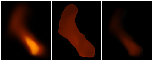
FLUID EFFECTS – clouds, fog, smoke, explosions
Depth can be emphasised by changing the density of the air eg fog’s colour, transparency, saturated distance, clipping plane and fine dust particles.
Need to specify the space where the effects will take place, called the container, a 2D or 3D space where the fluid is contained which can contain an emitter. The numerical density and velocity fluid property values in the Container portray the movement and shape of the fluid, the temperature acts upon the fluid to creates a reaction and density colour.
Container Properties: increasing the resolution increases the quality of the rendered fluid. Size defines the size of the fluid container in centimetres. Voxel resolution is defined through a grid, which are used to precisely control the container’s values.
CLOUDS: some things to consider – can use an emitter or a gradient painting the cloud particles as density with opacity adjusted in the brush settings along with Auto Set Initial State. Select the directional arrow in each axis of the container.
Containers attributes Lighting > Self Shadow > On and check Real Light to use the light in the actual scene. Shadow Opacity controls the degree of darkness in the clouds. Transparency in Shading of the fluidShape node adjusts the entire transparency and the Ramp under Opacity uses density to adjust transparency. Dragging the area to the right to make transparent areas of lower density, setting Opacity Input to Density and Interpolation to None. Areas of lower density are more transparent.
Under Textures in the fluidShape Node check Texture Opacity, choose the Texture Type. Amplitude adjusts the strength of the Noise, Ratio adjusts the Fractal Noise frequency, Frequency Ratio adjusts the frequency of the Noise to space, Depth Max determines the computation from Volume Nose Texture with higher values giving more detail. Can animate Texture Time of Texture Scale to create cloud movement.
FLUIDS: some things to consider – shaping the Emitter select Volume and Sphere. To activate gravity in the container set under Density the Density Scale 1, Buoyancy -1, Display section Numeric Display set to Density. Make the emitted particles collide with the surface. Under Surface set to Surface Render, Hard Surface. In Container Propertiers adjust the container’s resolution. UnderTextures for lava use Texture Incandescence. Shading has no Transparency, Glow Intensity to .2, set the colour to black, adjust the colours of the Incandescence Ramp Colour to show the lava colours of red, orange, yellow and black. Under Textures select Texture Incandescence then adjust Text Gain, Amplitude, Frequency Ratio and Dept Max.
PONDS: a ripple effect in a 3D container with a wake emitter which can be keyframed, also a Dynamic Locator or Make a Boat.
OCEANS: some things to consider – can create an Ocean Plane from the Fluids menu that automatically assigns an ocean shader to the plane. Attach to Camera. Using the Ocean Shader’s Attributes adjust the shape with the Scale, Wind UV, Wave Speed, Observer Speed to prevent overlapping waves, Num Frequence controls the frequency of the waves, Wave Length Min and Max randomises the height of the waves. For more random effects use the Wave Height and Wave Turbulence Ramp. Foam Emissions determines the density of the foam, Foam Offset applies foam evenly over any area. In Common Material Attributes adjust the colour of the waves, foam and reflective properties.
Surface movements, dynamic movements or boat movements can be set to follow waves. Depending on the speed and height of the waves an object may rise in the air or sink. Creating a dynamic locator will move along with the waves.
Water ripples, add a Preview Plane, adjust the Resolution, Create Wake creates a 3D container. The Volume Emitter can be attached to a Motion Path.
Lava Tutorial using Maya
Solidifying of Molten Lava
Introduction to Maya Fluid Effects Vol. 1
Introduction to Maya Fluid Effects Vol. 2
Create an Interactive boat simulation
A Maya Fluid Dynamics Quicksheet: Even though this was written for Maya 7, it maybe helpful for current versions of Maya.
Fluid Overview:
- Fluids are emitted into containers. When a fluid is emitted, it moves as if it were dye in a mass of liquid (which is, in a sense, what it is doing).
- A container is divided up into voxels, which are compartments of the container that store values for fluid dynamics. The visible parts of the fluid have a Density greater than 0. Nothing actually moves around in a fluid container, the voxels merely change their stored attribute values according to the simulation.
- A fluid can be 2D, 3D or just texture.
Things to keep in mind:
- Fluid emitters don’t really emit fluid. They emit properties. The fluid is already in the container. Heat and density are properties that can either be emitted by emitters or hand painted with the Paint Fluids tool.
- Fields should only be used for 2 or 3 frames before being keyed off. They can cause the fluid to behave erratically after that.
- Voxels should always be square or the fluid will look weird.
- To keep the fluid from moving after emission, set Density to
Static Gridor set Velocity to eitherOff(zero)orStatic Grid. - Maya 7.0 will use all available processors/cores to solve fluid dynamics, so spring for a multicore system.
- To improve renders, read this.
- Smoke has a sharp Opacity falloff, so make sure to adjust the Shading | Opacity curve and set Input Bias to around
0.5! - Do not render fluids with Production Quality! It will take forever. Instead, set that Render Globals option to
Preview Qualityand adjust the fluid’s render quality with Shading Quality | Quality. It will go much quicker with about the same results. - For texturing clouds and explosions, set Textures | Texture Type to
Perlin Noiseand check Textures | Inflection. This is a good place to start. - When scaling up fluidEmitters, reduce Fluid Attributes | Fluid Dropoff. When scaling them down, increase Fluid Dropoff. Apparently, Fluid Dropoff doesn’t scale well.
- If the fluidEmitter has been scaled in one or two axes and the fluid is only emitting from the center (instead of from the whole volume), then reduce Fluid Attributes | Fluid Dropoff until the fluid emits from the entire volume.
- For a puff of smoke or dust effect (at the footsteps of a character, for example), key fluidEmitter | Fluid Attributes | Density/Voxel/Sec and Heat/Voxel/Secto
0, then20for a few frames, then0again.
fluidShape Attributes
Where applicable, recommended attribute settings are specified in red. Nodes will be in bold italics. Attribute categories will be in bold. Attributes will be in italics(unless they are being defined in which case they are bold). Attribute values will be in fixed width. Heirarchies will use | (i.e. pipes) to separate parent and child (for example, fluidShape | Container Properties | Boundary X).
Container Properties
- Resolution – the higher this value is, the more detail and motion will be present in the fluid. Resolution is represented by values for x and y for a 2D fluid and x, y and z for a 3D fluid. This does not mean that a render will be low-res if Resolution is set low, but it does mean that its motion will be more general. A higher resolution allows for small eddies and more articulate motion.
- Size – controls the size of the fluid container. It is represented by x, y and z values. To keep voxels square, make sure that Size is in the same proportions as Resolution. If Resolution is
<<80,40,0>>then Size should be<<20,10,0>>or<<10,5,0>>, etc. - Boundary – if the value of Boundary X, Boundary Y or Boundary Z is
Both Sides, then the fluid will collide and interact with the borders of the container in that direction. If, for instance, the value of Boundary X is-X Sidethen the fluid will only interact with the container boundary in the -x direction. If the value of Boundary X, Boundary Y or Boundary Z isNone(or the opposite side is specified as a boundary), then the fluid will simply cease at the border. If the value of Boundary X, Boundary Y or Boundary Z isWrapping, then the fluid will wrap around to the opposite side.

Examples of boundaries and their effect on fluids.
Contents Method
- Density – the visible part of the fluid. Essentially, it is the “particles” of the fluid.
Off(zero)– the fluid is turned off (invisible).Static Grid– the fluid emits, but does not move after emission. No fluid calculations occur.Dynamic Grid– the fluid moves after emission. Fluid calculations occur.Gradient– fills up the entire container with fluid with the falloff determined by Density Gradient and Shading attributes. This is for non-dynamicapplications. Fluid will not move after it is set.
- Density Gradient – controls in which direction the gradient is applied.
 Examples of (from left to right)
 Constant, X Gradient, Y Gradient, Z Gradient, and Center Gradient.
- Velocity – pushes the fluid around the container.
Off(zero)– fluid dynamics are not calculated.Static Grid– the fluid emits, but does not move after emission. No fluid calculations occur.Dynamic Grid– the fluid moves after emission. Fluid calculations occur.Gradient– moves the fluid in the direction specified by Velocity Gradient.- Velocity Gradient – specifies the direction in which Velocity will occur. Only recommended for non-dynamic simulations.
- Temperature – moves the visible fluid around based on temperature. This attribute also affects color (the hotter a fluid is, the more incandescent it becomes).
Off(zero)– Temperature is not calculated.Static Grid– the temperature does not get pushed around between voxels. If heat is being emitted, it will remain confined to the emitter and not spread to fluid in any other area.Dynamic Grid– the temperature changes over the course of the simulation and will affect the fluid’s color. Useful for showing hot spots in smoke or simulating fire.Gradient– the temperature is static but has a falloff.
- Temperature Gradient – specifies the direction of the falloff of the temperature. It also controls in which direction the fluid will flow (if this value is
X Gradient, then in a 2D fluid the fluid will flow towards-xsince that’s where theX Gradientwould start).
- Fuel – determines the visibility and color of the fluid by controlling its “fuel source”. It requires a non-zero value in Temperature to show results.
Off(zero)– there is no fuel.Dynamic Grid– fuel will be emitted. This works with Temperature to determine if and when the fluid catches on fire (or changes color).Gradient– controls how the fuel is dispersed throughout the fluidShape. This would be useful to make sure that a fuel source does not move and ignite the rest of the fluid but still has a smooth falloff.
- Fuel Gradient – specifies the direction of the falloff of the fuel.
- Color Method – controls how the fluid is shaded.
Use Shading Color– the fluid is colored according to Shading | Color.Static Grid– not sure, yet.Dynamic Grid– the fluid will emit color according to the fluidEmitter | Fluid Attributes | Fluid Color value.
- Falloff Method – When set to
Static Grid, this attribute acts as a mask for the visibility of the fluid. The Paint Fluids Tool can be used to paint the areas in which fluid will be visible in the fluid container. New to Maya 7.0. For more info (if you have the Maya Help docs), go here.
Display
- Shaded Display – determines how the fluid appears in the viewports.
Off– no fluid is visible.As Render– fluid is shown as an approximation to how it will render.Density– the Density values of the fluid are shown as clear (for no density) and white (for full density).Temperature– the Temperature values of the fluid are shown as clear (for no heat) and white (for full heat).Fuel– the Fuel values of the fluid are shown as clear (for no fuel) and white (for fuel presence).Collision– white represents where a fluid is colliding with an object.Density And Color– shows Density and the unmodified static or dynamic color.Density And Temp– shows Density and Temp as RGB values where yellow represents the hottest areas within the density and blue represents the coolest areas.Density And Fuel– shows Density and Fuel as RGB values where yellow represents the highest concentration of fuel within the density and blue represents the lowest concentration.Density And Collision– shows Density and collisions as RGB values where yellow represents a collision within the density and blue represents no collision.
- Opacity Preview Gain – allows easier viewing of whichever attribute is being shown in Shaded Display. Turning this value higher turns up the opacity of the displayed attribute.
- Slices per Voxel – Determines how many planes are used per voxel in the viewport. A good value is 2.
- Voxel Quality – controls how the voxels appear in the viewport
Better– better appearance, lower performanceFaster– better performance, lesser appearance
- Boundary Draw – changes the way the fluid container is displayed. The displayed grid will have a number of divisions equal to the container’s resolution.
Bottom– displays only the grid on the bottom of the containerReduced– displays a frontface-culled grid. Recommended while editing the resolution of the container.Outline– displays a grid on all sides of the containerFull– displays a cube for each voxelBounding Box– displays only a cube for the container. Recommended once resolution is set.None– displays no container. Recommended for playblasts. Makes the fluid harder to select.
- Numeric Display – displays numeric values per voxel for various values.
None– displays no numbersDensity– displays the fluid’s density valuesTemperature– displays the fluid’s temperature valuesFuel– displays the fluid’s fuel values
- Wireframe Display – changes the way the fluid appears in Wireframe Mode
Off– no fluid is shownRectangles– displays each voxel as a rectangle. The lower the density, the smaller the rectangle.Particles– displays each voxel as a particle point.
- Velocity Draw – if checked, lines are displayed showing the direction in which the fluid is moving.
- Draw Arrowheads – if checked, arrowheads are drawn on the velocity lines.
- Velocity Draw Skip – a higher value here lowers the number of velocity lines drawn.
- Draw Length – controls the length of the velocity lines.
Dynamic Simulation
- Gravity – sets the gravity for the fluid. Should be kept at 9.8 for regular gravity (if basic unit is in meters) or 981 (if basic unit is in centimeters).
- Viscosity – sets the thickness of the fluid. 0 is like water and 1 is like tar.
- Friction – a value of one will significantly slow down any fluid that is colliding with an object. This will only work if Grid Interpolator is set to
hermite. It seems to have very little effect on the simulation, however. - Damp – lessens the effect of dynamics on the fluid. It is similar to Conserve in particles. A value of 1 will completely stop the fluid. Typically set to 0.005.
- Solver – determines the algorithm used to simulate fluid dynamics
none– no simulationNavier-Stokes– simulates underwater movement (eddies, etc.)Spring Mesh– good for surface water deformation (ripples, etc.)
- High Detail Solve – used to keep the fluid from diffusing too much during a simulation. Setting this to anything but
Offis useful for explosions, rolling clouds, and billowing smoke. New to Maya 7.0.Off– fluid will diffuse as normalAll Grids Except Velocity– similar toAll Grids(see below) except velocity is unaffected by High Detail Solve. This is useful to retain most of the benefits of the extra fluid cohesiveness without much of a higher calculation time. Do not set Grid Interpolator to _hermite if this is enabled.Velocity Only– enables extra cohesiveness for Velocity only. This is useful if there are artifacts due to high detail density solving with either theAll Grids Except VelocityorAll Gridssolving methods. Setting Grid Interpolator tohermiteis recommended for highly detailed results, albeit at the cost of a longer simulation.All Grids– enables the fluid to stay more cohesive over the course of a simulation. This will provide the most realistic and detailed fluid simulation if enabled. It will take twice as long to simulate than if High Detail Solve is set toOff. Do not set Grid Interpolator tohermiteif this is enabled.
- Solver Quality – controls how fine-tuned the solver is, I guess. New to Maya 7.0.
- Grid Interpolator – determines how the value changes of each voxel are interpolated (imagine a curve with each calculation as a keyframe).
Linearis quicker to calculate, but it’s less exact.Hermitewill produce more swirls in the simulation but is much slower thanLinear. - Start Frame – the frame in which the simulation will begin. If Start Frame is set to a value lower than your playback range’s first frame, then the simulation will continue to run once it has run beyond the playback range’s last frame (instead of returning to the beginning of the playback range and restarting the simulation). Another point to keep in mind is that even if the fluidEmitter is keyed to begin at a particular frame, the scene will still solve for the fluid as long as the current frame is past the Start Frame. This means the scene will run slow even if nothing is apparently happening in the fluid.
- Simulation Rate Scale – controls how fast the simulation plays out. The higher this value, the faster the simulation goes. This is useful for creating roiling smoke or explosions. It is recommended to start working with the fluid with a Simulation Rate Scale of
1or2, and step it up as needed. Explosions tend to use a value from8to12. Values higher than16may produce unpredictable results. - Disable Evaluation – checking this will disable the simulation.
- Conserve Mass – doesn’t do much anymore. Ignore it if you wish.
- Use Collisions – toggles fluid collisions with objects.
- Use Emission – toggles the emitter on and off.
- Use Fields – toggles whether fields will affect the fluid or not.
Contents Details
- Density
- Density Scale – scales the initial density value that is placed in each voxel. While this controls the apparent transparency of the fluid, it is best left at
0.5. The transparency should be driven by the Shading | Transparency attribute instead. - Buoyancy – determines whether the fluid is more buoyant and floats upward or is less buoyant on settles downward. A value higher than one will speed up the vertical movement. Negative values cause the fluid to move downward.
- Dissipation – causes the fluid to disappear at a point where it is most likely to dissolve into the surrounding fluid. It works a bit like Lifespan works in particles.
- Diffusion – causes the fluid to spread out into the surround fluid and soften at the edges.
- Density Scale – scales the initial density value that is placed in each voxel. While this controls the apparent transparency of the fluid, it is best left at
- Velocity
- Velocity Scale – scales the strength of the velocity in x, y, and z. If, for instance, the y value is changed to
0.5, then the fluid will move upwards half as fast as it would otherwise. This value should generally be between0.8and2.0for acceptable results. - Swirl – causes the fluid to swirl. A higher value means more swirling. This is useful for roiling clouds or explosions.
- Velocity Scale – scales the strength of the velocity in x, y, and z. If, for instance, the y value is changed to
- Turbulence
- Strength – brings more turbulence into the fluid. Note that this is built into the fluid. It can be used alongside the Turbulence field.
- Frequency – changes the size of the turbulent waves. A lower values produces larger waves than higher values. The default setting of
0.2tends to create a large swirling motion that fills the entire fluid container. - Speed – higher values speed up the turbulence calculations. This doesn’t mean, however, that the fluid will move faster; it just means that there will be different points along the turbulence wave by which the fluid will be affected. Consider it more of a seed.
- Temperature
- Temperature Scale – scales the heat of each voxel.
- Buoyancy – similar to *Density*|_Buoyancy_, except it affects the temperature.
- Dissipation – similar to *Density*|_Dissipation_, except it affects the temperature.
- Diffusion – similar to *Density*|_Diffusion_, except it affects the temperature.
- Turbulence – applies a turbulence to the area an emitting fluid occupies and not to the entire fluid container (as Turbulence does). Useful for explosions and fires.
- Fuel
- Fuel Scale – scales the fuel value of each voxel.
- Reaction Speed – a lower value will cause the fuel to ignite much slower. Up this value for faster-burning fuels.
- Ignition Temperature – controls the point at which the temperature is hot enough to ignite the fuel (i.e., cause the incandescence colors to kick in).
- Max Temperature – affects how hot the fuel will burn, and, in turn, affects the color of the fluid. Lowering this value will keep the fluid from reaching the higher end of the incandescence ramp.
- Heat Released – controls how much heat is released from the fluid. It affects the color of the fluid.
- Light Released – controls how much light is released from the fluid. It affects the incandescence of the fluid.
- Light Color – sets the incandescent color that Light Released affects.
- Color
- Color Dissipation – this is enabled only when *Contents Method*|_Fuel_ is set to
Dynamic Grid. It controls how quickly the color goes to black. - Color Diffusion – this is enabled only when *Contents Method*|_Fuel_ is set to
Dynamic Grid. It determines how much the fluid color blurs at its edges.
- Color Dissipation – this is enabled only when *Contents Method*|_Fuel_ is set to
Grids Cache
These options control which values get cached. To cache Fluids, go to Fluid Effects > Create Cache. These same options are in the Create Cache option window. The attributes are self-explanatory.
Surface
- Volume Render/Surface Render – if Volume Render is on, then the fluid will render out with a falloff. If Surface Render is on, then the fluid will render as a solid mass with no falloff. Surface Render is very slow, even when editing attributes. Its best to enable this after all settings have been finalized.
- Hard Surface/Soft Surface – only enabled if Surface Render is on. If Hard Surface is on, then it will render the way it appears on screen. If Soft Surface is on, then it will render like the Hard Surface, except with a falloff around the outside edges.
- Surface Threshold – only enabled if Surface Render is on. This determines where the fluid’s surface will appear within its volume. Higher values shrink the visible fluid.
- Surface Tolerance – only enabled if Surface Render is on. It doesn’t seem to do much. Supposedly, a lower setting will render better, while a higher setting will render faster.
- Specular Color – only enabled if Surface Render is on. This affects the surface in much the same way that a Blinn shader would.
- Cosine Power – only enabled if Surface Render is on. This affects the surface in much the same way that a Blinn shader would.
 From left to right, the following renders use Volume Render, Surface Render with Hard Surface, and Surface Render with Soft Surface.
Environment
Creates an environment map for Surface | Specular Color.
- Refractive Index – controls how “wet” the surface looks. Lower levels (less than
1.0) make the surface look like water. Supposedly.
Shading
Shading and Texturing will ultimately determine how the fluid will render out.
- Transparency – controls the transparency of each voxel of the fluid. A value of all black means no transparency. A value of all white means full transparency. This should not be confused with Opacity, which affects the fluid as a whole, and not each individual voxel.
- Glow Intensity – works the same as Glow Intensity for shaders (i.e., it’s a post-process effect). This effect can be controlled by the Shader Glow shader.
- Dropoff Shape – the shape within the fluid container beyond which the fluid disappears. For example, if Dropoff Shape is
Cube, then the visibility falloff is in the shape of a cube. If it isSphere, then the falloff is in the shape of a sphere (centered in the middle of the container). This is useful for fading out a fluid before it reaches the edges/sides of its container. Dropoff Shape will not affect any edge or side that is set with a boundary ofNoneorWrapping - Edge Dropoff – controls how far from the edge or side that the falloff begins.
- Color – determines the base color of the fluid. The darker this color is, the more effect Incandescence will have on the color of the fluid.
- Selected Position – the position of the currently selected color point in the color ramp to the right. The left side of the ramp is 0 (coloring voxels with a value of 0 from Color Input) and the right side of the ramp is 1 (coloring voxels with a value of 1 from Color Input).
- Selected Color – the currently selected color point’s value.
- Interpolation – the type of smoothing that occurs from one color point to another. These are similar to tangent settings for keyframes on an animation curve.
- Color Input – determines which value or attribute drives the color of the fluid.
- Input Bias – shifts the values provided in Color Input by the given amount. For example, the color ramp is red on the left side and green on the right, and the Color Input is
Density. With an Input Bias of0, all voxels whose Density is0would be red (at least they would be if they weren’t invisible) and all voxels whose Density is1would be green; any values in between are interpolated. Now, if Input Bias were0.5, then all Color Input values (which in this case is driven by Density) would be adjusted by 0.5 (values above1would be clamped at1). All voxels whose Density is0would have a Density of0.5(but only for the purposes of determining the color!). Voxels with a Density greater than1would be clamped at1. That means that all other Colorvalues will be mapped between0.5and 1.0= on the color ramp. In this case, the least dense areas will be colored red-green (0.5on the color ramp) and the most dense areas will be colored green (1.0on the color ramp).
- Incandescence – brightens Color using color values from the Incandescence ramp. This is most useful when Color is a dark value.
- Incandescence Input – determines which value or attribute drives the incandescence of the fluid. For explosions and fire, it is recommended to keep this at
Temperature. - Input Bias – this attribute is comparable to Color | Input Bias, except it adjusts the incandescence of the fluid.
- Incandescence Input – determines which value or attribute drives the incandescence of the fluid. For explosions and fire, it is recommended to keep this at
- Opacity – controls the opacity of the fluid as a whole using a falloff curve. To better visualize how the falloff graph works, imagine that the dark gray part is the visible fluid and the light gray part is the invisible fluid. The left side of the graph would represent the falloff of the visible fluid’s opacity. In the example below, the left image has a linear falloff while the right image has a more rounded falloff (which is why the outer edges of the fluid look thicker).

Displayed is how Opacity affects the fluid. The insets are the Opacity falloff graph.
-
- Opacity Input – the attribute or value used to determine how opaque voxels are. The recommended setting is
Opacity. - Input Bias – this attribute is comparable to Color | Input Bias, except it adjusts the opacity of the fluid.
- Opacity Input – the attribute or value used to determine how opaque voxels are. The recommended setting is
Shading Quality
If the fluid renders with artifacts, try adjusting these values to fix it.
- Quality – controls the quality of the aliasing in the fluid’s render. It is recommended to use this attribute to improve the fluid render and not the Anti-Aliasing Quality attributes in Render Globals. Upping Quality will get rid of some of the aliasing artifacts that appear in fluid renders.
- Contrast Tolerance – this is supposed to weight the render towards better contrast or faster rendering, but it appears to cause no noticeable differences.
- Sample Method – the method used to sample color ranges for rendering.
Uniform– even sampling throughout the image.Jittered– gets rid of banding, but applies more noise.Adaptive– gets rid of noise, but applies more banding.AdaptiveJittered– combines the best traits ofAdaptiveandJittered.
- Render Interpolator – if this is set to
linearand the fluid renders out with sharp contrasts, then set this tosmooth.
Textures
 This is where most of the visible changes in the look of the fluid is made. Do not underestimate the power of textures!
- Texture Color – places a texture on the fluid’s color (Shading | Color).
- Texture Incandescence – places a texture on the fluid’s incandescence (Shading | Incandescence).
- Texture Opacity – places a texture on the fluid’s opacity (Shading | Opacity).
- Texture Type – defines which algorithm is used to texture the fluid. Examples of the options are provided in the image below.
- Coordinate Method – not sure what this does.
- Coordinate Speed – nor this one. But if I had to guess, I think it would control UV texture scrolling.
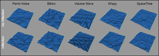
Examples of fluids textured with various texture types.
- Color Tex Gain – controls to what degree the texture will affect the color. A value of
0means that the texture will have no influence over the color. Any value above one will increase the effect of the texture on the color. - Incand Tex Gain – similar to Color Tex Gain except it applies to Incandescence.
- Opacity Tex Gain – similar to Color Tex Gain except it applies to Opacity.
- Threshold – raises each value in the texture by the specified amount, clamping at
1.0, and re-interpolating the values in-between. Visually, it raises the floor of the texture so black becomes shades of gray. - Amplitude – acts as a multiplier to the max height and depth of the texture. Raising this value will increase the distance between the lowest values and highest values.
 When creating smoke, treat this value as ambient occlusion. Raising it will heighten the effect as well as increase the fluid density.
 - Ratio – seems to add more relief to the texture. It’s effect is similar to that of Amplitude.
- Frequency Ratio – this attribute will repeat the texture dynamically and fit it to the fluid container. It acts much like increasing the Repeat UV value of a Texture 2D node except the pattern isn’t repeated in quite the same way.
- Depth Max – increases the amount of relief in the texture. More pits will be added (i.e., subtractive values).
- Invert Texture – reverses the value of the texture color (black becomes white and white becomes black).
- Inflection – adds an uneven aliasing over texture edges. It also changes the texture in some other manner. Examples of the differences between Inflection on and Inflection off are in the image above.
- Texture Time – used to animate the texture or make positional adjustments. To animate the texture, key this attribute over time. The animation that occurs depends on the value of Texture Type.
- Frequency – this is similar to Frequency Ratio, but it doesn’t change the relief of the texture, it just fits more of the texture in the same amount of space while proportionately re-scaling it. When the value is increased, the texture appears to shrink.
 When Texture Scale is changed, Frequency should be changed proportionately (unless getting the texture to look very different was the point of the change).
 - Texture Scale – scales the texture according to the given values.
- Texture Origin – moves the origin from the center of the container by the given coordinates. This value will be relative to the center of the fluid container. Animating this in a particular direction can make the fluid appear to move (if Texture Opacity is checked).

- Implode – when this is a positive value, the center is shrunk and the outer edges are pulled outward.
- Implode Center – the center of the Implode effect relative to the center of the fluid container.
- Billow Density – only available if Texture Type is
Billow. This attribute changes the Billow texture from mere bumps to rolling hills. The only valid range is from0to1. - Spottyness – only available if Texture Type is
Billow. It slightly alters the texture by some unknown method. - Size Rand – only available if Texture Type is
Billow. Raising this value will decrease the size of the “hills” and remove much of their overlapping. - Randomness – only available if Texture Type is
Billow. Setting this to0will display a repeated pattern. Setting this to any other value up to1will increase the randomness of the pattern. Values greater than1and less than2seems to have a similar effect to Size Rand. - Falloff – only available if Texture Type is
Billow.Linear– standard setting.Smooth– this setting smooths out the texture.Fast– increases the texture detail.Bubble– turns the texture into a mass of ridges.
- Number of Waves – only available if Texture Type is
Volume WaveorSpaceTime. When Texture Type isVolume Wave, raising this value will smooth out the texture while attempting to keep the minimum and maximum values. There seems to be no effect when Texture Type isSpaceTime.
Lighting
- Self Shadow – check this so that the fluid will cast shadows on itself. Renders with this option will take about 33% longer.
- Hardware Shadow – check this so that the self-shadowing is visible in the viewport.
- Shadow Opacity – a value of
0causes transparent shadows and a value of1causes fully opaque shadows.
- Real Lights – check this to use the scene lights to render the fluid
- Directional Light – if Real Lights is unchecked, then the fluid will render with a default directional light. This attribute assigns a directional vector to that light.
fluidEmitter/wakeEmitter Attributes
Where applicable, recommended attribute settings are specified in red. Nodes will be in bold italics. Attribute categories will be in bold. Attributes will be in italics(unless they are the being defined in which case they are bold). Attribute values will be in fixed width. Heirarchies will use | (i.e. pipes) to separate parent and child (for example, fluidShape | Container Properties | Boundary X).
Basic Emitter Attributes
These are much like particleEmitter basic attributes.
- Emitter Type – the method by which the fluid will be emitted.
Omni– fluid is emitted in all directions.Surface– fluid properties are randomly distributed onto a NURBS surface.Curve– fluid properties are emitted onto a curve.Volume– fluid is emitted from a primitive volume.
- Cycle Interval – restarts the random number of streams after a given frametime
None (timeRandom off)– no restart occursFrame (timeRandom On)– randomization streams restart after the given number of frames. This will most likely not be a seamless transition.
- Min Distance / Max Distance – enabled when Emitter Type is
Omni. These attributes provide the start and end distance from which the fluid will emit.
Fluid Attributes
- Density/Voxel/Sec – the density of the emitted fluid. Requires fluidShape | Contents Method | Density to be
Dynamic. - Heat/Voxel/Sec – the temperature of the emitted fluid. Requires fluidShape | Contents Method | Temperature to be
Dynamic. - Fuel/Voxel/Sec – the fuel of the emitted fluid. Requires fluidShape | Contents Method | Fuel to be
Dynamic. - Fluid Dropoff – determines how much the density of the emitted fluid fades as it is emitted near the outer surface of the volume emitter. Note that this attribute does not scale when the fluid container is scaled. It will have to be manually adjusted to maintain the same falloff ratio.
- Emit Fluid Color – check this to allow the fluid to emit the fluid’s color. This requires fluidShape | Container Method | Color Method to be set to
Dynamic Grid. - Fluid Color – the color of the emitted fluid (if Emit Fluid Color is checked). This value should probably be keyed or mapped if the intention is to use dynamic color. Most coloring effects can be accomplished easier if fluidShape | Container Method | Color Method is set to
Use Shading Method. - Jitter – not sure what this does. Probably jitters or something.
Fluid Emission Turbulence
- Turbulence Type – the options are
GradientandRandom, but there seems to be no real difference between them. - Turbulence – increases the randomness of the turbulence.
- Turbulence Speed – affects how often the turbulence will change over 1.0 / Turbulence Speed seconds.
- Turbulence Freq – determines how smooth the turbulence is. Values around
0will really smooth the turbulence out, whereas higher values seem to have very little effect. - Turbulence Offset – translates the turbulence. This can be keyframed for a blowing turbulent wind effect.
- Detail Turbulence – adds a second layer of turbulence to the surface of the pond. Its value is the intensity of that secondary turbulence (which will always be faster and more frequent than the primary turbulence). For more control, set this attribute to
0and create a second emitter for secondary turbulence.
The Fluid Effects Menu
Some of the options are self-evident, so those won’t be covered.
- Add/Edit Contents
- Emitter – adds an emitter to the currently selected fluidShape.
- Emit from Object – creates a surface emitter for the currently selected fluidShape from the concurrently selected object.
- Gradients – replaces the values of fluidShape attributes with the various gradients.
- Paint Fluids Tool – allows painting in fluids. This is useful for painting in a general fluid shape for an initial state or for painting in a falloff map.
- With Curve – turns a curve into a paint stroke (like Paint Effects) for the specified fluidShape attributes.
- Initial States… – this isn’t all too useful. The current fluid’s resolution can be set to match that of an example file or vice-versa.
- Get Fluid Example…/Get Ocean Pond Example… – his will open up sample Maya files of pre-created fluid effects.
- Ocean – does ocean stuff. Not covered, yet.
- Pond – does pond stuff. Not covered, yet.
- Extend Fluid – changes the size of the fluid container by adding and subtracting voxels. This means that the size of the container and the resolution are being changed in proportion to each other.
- Edit Fluid Resolution – only useful when it is necessary to rebuild the resolution of the initial state (since changing the resolution within the fluidShape node will delete the initial state).
- Make Collide – allows fluids to collide with an object. Select the object, then select the fluidShape and run this command to create collision objects.
- Make Motion Field – creates a field that will push fluids in its motion path away. It may also work with particles (though it is unavailable form the Particlesmenu).
- Set Initial State – sets the value of each voxel at the start of the simulation to the current state.
- Clear Initial State – clear the above state.
- Save State As… – save the current state as a MEL file. To bring that state back, import the MEL file using File > Import… If the state saved was an initial state, then it will import as an initial state (as opposed to disappearing if you go back to the start of the simulation).
- Create Cache – store the fluid calculations so they don’t have to be re-calculated next time the sim is run. The option box allows the caching of certain attributes to be turned off.
- Cache File Format – choose
Single Fileif your cache is under 2GB, and chooseOn File per Frameif your file would be 2GB or over. - Sampling Rate – higher values allow fast-moving fluids to render less spotty.
- Cache File Format – choose
- Append to Cache – if a cache is already created, the cache must be appended to.
- Replace Cache Frame – replace the current frame’s cache with the current frame’s value.
- Truncate Cache – cuts the cache down to whichever frames were cached before the current frame.
- Delete Cache – supposedly deletes the cache file. Sometimes an error may show up during render that more than one cache file is present. This may be due to the cache file not being physically deleted by Windows. Instead of using Delete Cache to get rid of a cache that will be replaced, use Truncate Cache to truncate it on the first frame.
Redshift 2 Maya – Tutorial #1 – Particle Rendering
Making a Spalsh with RealFlow and Maya Tutorial
Maya Dynamics Tutorial – Galaxy Particle Effects HD
Maya – Basic Particle Dissolve Effect
DYNAMICS 002
REPORT 2B: Schooner, Sail Boat

Starting on this adventure, translating my sailing research into dynamics was not off to a good start. When moving the sail boat the pieces of the model were not staying together, not even when grouped.
Then the nCloth would not work on the sails.
Dynamics 101 – the model has been constructed from nurbs, before being able to consider translating some of my research about sailing, wind and oceans into dynamics I am going to need to get some basics happening.
To get started a poly hull has been created enclosing the bulk of the schooner model, then grouped, keeping the model together and enabling the dynamics to work.
The sails have been remade as poly planes,1 for width and height subdivisions then smooth mesh, 3 or 4 subdivisions. I was still not meant to get started on the sailboat project, I was creating too many subdivisions, like 8 and the system was crashing. The lofted surfaces and some of the nurbs geometry around the sails has been deleted, not being needed to connect the sails or seen in the shot.
 We used dynamic constraints for the dress exercise in class and using them to attach the sails to the booms and masts. Initially, started by converting a couple of the nurbs masts and booms from nurbs to polys then using component to component constraints with a separate nCloth for each sail. Vincent’s wisdom prevailed using Transform nConstraints, meaning I did not need to convert the model from nurbs to polys to use nConstraints and all the sails became the one nCloth resulting in more efficient processing.
Starting to work and get things happening.
I used a heavyDenim preset in an attempt to replicate the feeling of the weight of sails. When we did the dress in class the presets made a difference . Then I created a shot camera, changing the Far Clip Plane and key framed the boat over 100 frames. Still getting the basics, as it was not going to be animated, it is going to move in the ocean dynamically.
Now to keep it all together, I forgot a few more basics, like play the simulation and not jump to the end to see what is happening and the Playback Speed, Play Every Frame, Max Real Time.
The nConstraints > Transform Constraints to connect the corners of the sails to the masts, booms and ropes was starting to work and there is a little locator that can be parented to the relevant geo. At first I was using a separate constraint for each sail’s corner and parenting to the relevant parts of the sailboat

Getting the constraints to work took several attempts, working out where to connect the sails so they started looking like they were connected to the boat. It went from one on each corner to a couple at the corners of the sail’s edge, then finally some parts of the sails needed the whole side constrained using an edge instead of a vert. The sail is now staying firm along the relevant booms and ropes giving a more realistic connection.
The constraint locator is relevant to where it is parented and if the locator is changed it needs to be done on frame one.

Following the research I have done, the sails needed to be positioned about 45 deg to the boat with each boom at a slightly different angle so the sails can utilise the winds.

Grouping the relevant model parts and moving the pivot point of the group to animate and move the booms meant revisiting the Transform Constraints. Chaining the parts of the boat where the constraints had been parented, string Constrain Method and now the sails are connecting and working better with the model.
You can create a Transform constraint to hold specific nCloth components in place or move them through XYZ space. For example, you can make a Transform constrained nCloth follow its animated passive object through its scene by parenting its Transform constraint locator to the passive object.
dynamicConstraintShape: http://knowledge.autodesk.com/support/maya/learn-explore/caas/CloudHelp/cloudhelp/2015/ENU/Maya/files/GUID-1609C235-5031-4D06-A94C-82E8A76B8726-htm.html
At this point I made a basic ocean, through the shot camera so it would scale based upon the camera distance, to see how it might all work. The ocean is generating movement, not the actual ocean which is not dynamic, a shader has been created and is procedurally creating the ocean and the shader is driving the movement. Simulating the rolling oceans, waves and wakes created by boats and later using bifrost to include these ocean details around the boat as it moves.
The next problem I had was the scale, not the first time my brain has needed to get around this issue. Scale and Dynamics are inseparable, the model was about 8000cm and the sail boat was not moving on the ocean. There was also a problem with the sails, the speed of the fall of dynamic objects, it was all over the place and part of the solution for the sails was the scale attributes.
Ocean Shader Scale = 0.001 is 0.0001 seen in script editor. Looked at the scale for the whole solver, nucleus and the Space Scale to 0.1 Everything to scale now, ocean scale matches the boat.
Now working on the shape of the sails, to look like they were sailing. A big factor was the nCloth’s dynamic property of Input Mesh Attract, nCloth has an original and dynamic mesh where the relationship with the original curve can be adjusted.
FX > both > paint vertex properties > input mesh attract
With an Input Mesh Attract is like using goal weights, a value of 1 means the meshes stay with each other, for 0 the shapes move apart. The Input Mesh Attract can be painted, using values between 1 and 0 or white and black to vary how the meshes either stay or move apart.
The boat – another beginners idea, animating the boat, really – totally forgot about moving it dynamically. Selecting the boat then the ocean, creating a dynamic boat with a locator for the dynamics, the locator is the true boat and is dynamic and positions the boat. Maya works out the dynamics with the boat length and width for how it is interacting with the ocean.
Now the boat is totally in the wrong place and not moving, not even a fraction of a fraction. Adjusting the Buoyancy of the locator controlled the floating of the boat, now to move it.
The throttle drives the animation and it has been adjusted at various stages to fit in with the size, shape and movement of the ocean and waves creating a more realistic feel and look. Initially there was too much bobbing up and down with the boat looking like a toy in the ocean. Changing the values in the throttle’s expression when adjusting the ocean shader’s values combined to create a more realistic look.
One of the biggest problems I had was having sails look like they were capturing the wind to drive the boat forward, the arc shape of sails. Using fields was not working, the constraints and painted weights were having more control of the sails movement regardless of hanging values such as direction, magnitude, attenuation and speed.
Then looking at the values on the nucleus for gravity, direction, air density, wind speed, direction and noise again I could not see any visible different from what the constraints and painted input attract was doing. I was not able to use these attributes to have the sails look like the wind was driving the boat with the sail’s shape. It was ok to use the nucleus as there were no other dynamics in the scene that the nucleus would affect.
My initial idea was to set the sails to look like my research and reference using Set Initial State and to start the sequence at this point. Because I’m not happy with how the sails are looking I have not set an initial state, animating the booms with the sails dynamically attached and moving as part of the dynamic simulation.
Now some more fun, the ocean. The waves were too big, too similar for the ocean and moving around too much for what I was aiming for. The values I experimented with were scale, turbulence, frequency, wave speed, wave length, wave height, wave peaking, min/max, wind uv, wave direction, wave direction spread, and dampening.

I did not need to adjust collisions as there were no problems here as the boat model with the dynamic movements and between the dynamic sails were not colliding, this included no issues with collision thickness.
Finally I added a physical sun and sky, adjusting the horizon and turned off primary visibility in the render stats for the polyHull.
This is an interesting subject and a new and developing area of 3D. While continuing to work on this project I have been able to cover many of the basics we covered and look forward to building on this.
There were areas I researched and learnt about which have not come to pass in my simulation due to learning and time constraints.
This has included using nHair’s dynamic curves for the ropes, considering curve thickness, collide with offset, stiffness scale, stretch resistance, start curve attract and matching the original cure. nCloth and nHair can interact with each other having a unified solver. Also playing with clouds in the sky and some atmosphere above the ocean, all ideas we have explored in class. This is going to be an adventure of another day.
I was looking forward to a more realistic simulation and including a bifrost guided simulation, I checked it out and did not have the time at this point and needed help going through the process.
Some of what I explored for the bifrost guided simulation was to created a poly disc approxmetly the same size as the ocean > assign ocean shader > selected a face (must use this face, cannot just go and make another one, to do with how the texture and how the uv’s are laid out, cannot use the preview plane, not sure geo, different node). Edit Mesh > duplicate, child of original plane. Smooth mesh with 8 divisions > delete history > assign ocean shader to the face, same shader so the uv’s match up. Select plane then shift select the ocean shader > modify > convert displacement to polygons with history. Has displacement on it now and can use for the wakes on the ocean, a piece of geo to deform like an ocean and can now use a guided simulation, making the geo the guided simulation. Create a container and make passive collider.
This cannot be scaled and moved and needed to make it where I want it, where the boat is moving on the ocean.

I was not able to play the dynamic simulation, they system could not handle it and kept crashing. The issues here for the bifrost was I needed to make an alembic file, would take about an hour as it is creating a mesh for each frame and to also scale the whole scene as it will not work with real world scale in order to make this work.

Rendering takes a long time, with bifrost being rendered separately and then to be comped in for the final playback.
I look forward to the day when I am more confident and skilled to be able to understand, find the buttons and implement the knowledge I am reading.

Naming for the Schooner:
Front – Bow
Back – Stern
Left, when facing Bow – Port
Right, when facing Bow – Starboard
Fore Mast
Main Mast – the tallest one
Boom
Flying Jib
Outer Jib
Inner Jib
ForeTop Sail
Fore Sail
Main Top Sail
Main Sail
Maya 2011 Basic nCloth Dynamic Constraint Tutorial by Stuart Christensen
Dynamic Rope Bridge – Maya
Bifröst GUIDED SIMULATION
New guided simulation workflows let artists drive the behavior of liquids using a cached simulation or an animated mesh object. With a guided simulation, a full-depth low-resolution liquid can be used to guide a high-resolution simulation on the liquid’s surface. Use guided simulation for such effects as carefully art directed hero waves. Artists can perform multiple iterations at high resolution while retaining the basic look and motion of the underlying guiding simulation.
Autodesk Knowledge Network: Guide a Bifröst simulation of a liquid surface
Autodesk Maya 2016: Bifröst Procedural Effects Platform presentation by Daryl Obert
Maya Features: Dynamic simulation and effects
Arnold for Maya user guide Bifröst
Bifrost: Exclusive first in-depth look By Mike Seymour March 18, 2014
BIFROST
Create an Explosion Using The Aero Solver in Maya Bifrost
AREA Welcome to Valhalla, your source for Bifrost-related tutorials, techniques, tricks, hacks and ideas! by Adrian Graham
A Maya Fluid Dynamics Quicksheet
SAILBOAT in the OCEAN
For this assessment students will be required to present a plan for the Sailboat in the Ocean dynamics project. This plan will take the form of a written report, including Research and Development and Reference Material with images and videos.
I started my research into this project by looking at sailing. What factors cause a sailboat to move the way it does? Then I looked at how are these elements are created in the environment, while considering how this effect might be created with the dynamics we have covered together with further research to include some areas not yet covered.
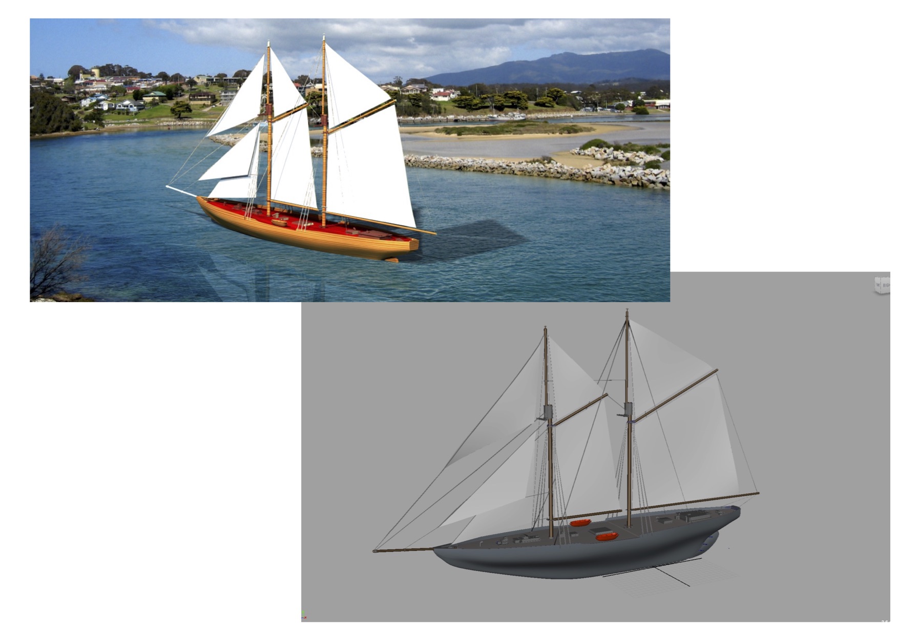
supplied reference and shot of supplied 3D model
Still Reference from the Internet:
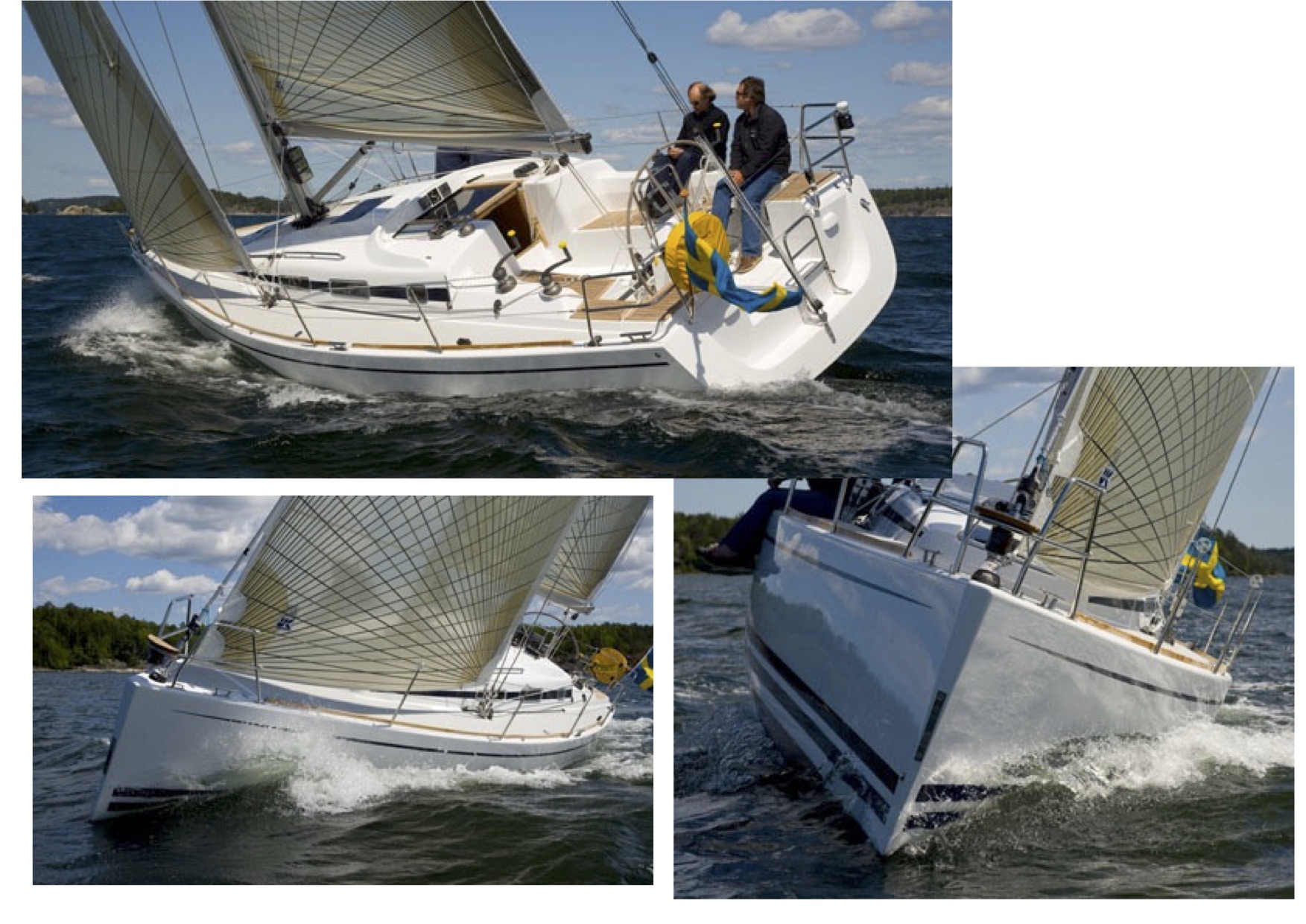
Youtube visual reference at the end under reference.
It is a slightly cloudy day, bright sunshine, light winds with slightly choppy though gentle smaller waves and a little foam on the top.
What is the role of the weather in how the air and ocean behave?
The high pressure areas move anticlockwise and low pressure areas move clockwise generating wind and the closer they are the stronger the wind will be.
Wind is a major factor in how waves are formed and the random distribution of wind pressure blowing across the surface of the ocean creates a certain amount of wave randomness.
As the winds blows longer and stronger the small waves become larger and faster, the interactions between the waves on the surface generate greater wave action, creating a range of height, duration and shape. The strength (intensity), duration (how long it blows) and fetch (distance) of the wind determines the wave formations. Land mass also affects the winds, offshore winds blowing from the land towards the ocean combine with the onshore winds blowing from the ocean towards the coast combining to affect the winds.
The speed of the waves are controlled by gravity, wavelength and water depth, including variances in the ocean floor. Initially, in the ocean, the waves are more vertical in shape then travelling toward the shore they move faster above the water line and as the ocean depth decreases the upper part of the wave begins to tilt forward.
Now I ask how does the wind and water move the sail boat?
I went looking at the weather forecast for Sydney, North Head, confusing or helpful? Confusing.
Strong wind warnings of more than 25 knots or nearly 50kmh, not releasing time for sailing. MODERATE SEAS AND WINDS
Mostly sunny. Winds west to southwesterly 20 to 30 km/h.
Wind 18 W, Waves 1.2 M, Wave Period 6.7s SW, Wave Height 4’ 2” feet
North Head Average 6 WNW, Gust 10 WNW
 Back to moving the sail boat: thinking of the sails, there is also the keel and the rudder.
Boats can sail with very little wind, how? Consider the wind direction, sailing downwind or parallel to the wind, catching the wind in the sails and sailing slower than the wind. Sailing upwind or anti-parallel to the wind which is impossible with conventional sails, resulting in sitting there with the sails flapping.
Sailing at 40° or typically 45° to the wind, tacking (alternate lines on either side of the wind direction) and they can go where they like.
From what I found this is about the wind generated by the boat moving or boat wind, the wind from the weather or true wind and the in-between or apparent wind which is between the boat wind and the true wind. The idea is for the apparent wind and the sail to be parallel, giving lift and drive on either side of the sail or sailing at 45° to the wind.
How a Boat Sails in Apparent Wind
The sail has a forward facing curve, not too too deep or too abrupt otherwise the air will stop following the curve of the sail and the sail shape, its curvature generates the lift.
Now there is the keel, the sail in the water, giving the ability to sail against the wind in certain directions and giving a balance of forces with the sails. With equal sideways pressure from both sides, the sails and the keel, they cancel out and leaves the forward movement.
How do I start to translate these concepts into the dynamic motion of the sailboat in the ocean using Maya’s dynamic tools. I need to consider the sails, ropes, masts, booms, ocean and the movement of the boat.
Some ideas from what we have learnt in class.
For the sails, there are a couple of options that we explored in class. The class exercise and the rolling ball through the curtain.
Make the sails nCloth using one of the presets for the fabric.
One way to connect the sails to the structure would be with nConstraints
between selected vertices of the nCloth and the geo. Selected edges of the sail can use a method like Rubber Band or Spring and attributes such as Strength, Glue, Bend, Friction and Rest Length to fine tune how different areas of the sails behave where they are attached to boat.
Another option was using painted weights values on the fabric, making different parts of the sails more or less dynamic. The fabric was bound to the joints, locators can be used for binding, then using the Input Attract to connect the nCloth’s original and dynamic mesh, creating the dynamic effect. This might be over kill for the sails and possibly nConstraints will be enough.
To represent the effect of the wind on the movement of the sails there are fields such as air and turbulence.
nHair’s dynamic curves would be used for the ropes, masts and booms which are light weight for simulations. There are two curves, first curve is static and the second curve is the dynamic curve. The length can be locked and there are attributes for Collisions, Stiffness Scale, Start Curve Attract and the Dynamic Properties.
When we made the snake in class we used our own dynamic curve with the joints following the curve’s movement. We used joints and not sure if this would work with locators for an IK Handle. The thought here is that if joints are created then could they also be used for the sail’s painted weights? Again it might be overkill for what is needed to be achieved.
Reading more about constraints between vertices and other objects, which can be locators and can then be animated or possibly parented or constrained to the ships geo as the ship moves around the scene.
I am not sure how the collisions will work between the sail boats geo. The sails are nCloth, then would they be rigid when interacting with the nHair of the ropes. I have read about how layers can be used to control how objects collide and collisions can be painted. There is the option of two nucleus systems that do not interact, then how would the field work between them? Maybe look at the Substeps and Collision Iterations to see how this works. I need to think about this a bit more.
Now the Ocean, which we have had an introduction to in class so the following including the use of Bifröst is based on my reading.
Fluids in Maya consists of containers with emitters or painted attributes and an ocean shader which is used to realistically simulate rolling ocean waves, ripples in ponds and wakes created by boats. The shader system is not part of the Nucleus system, even though fluid containers take less time to calculate the shader option is more suited to the needs of creating an ocean where objects can float on the surface and react to the motion of the water.
The ocean is being created with Maya’s 2008 academy award winning Fluids, created by Duncan Brinsmead. Its Ocean shader behaves dynamically and uses an animated displacement map to create the realistic ocean or water surface. This includes wakes, which is a fluid container with a spring mesh solver and the emitter being used to drive the motion of the wake fluid adding additional displacement and/or foam to the Ocean shader. Objects can be floated using different types of fluid locators. Adjustments can be made to the Wave Speed, Observer Speed, Wave Length Min and Max, Wave Height, Wave Turbulence, Wave Peaks, Water and Foam Colour, Trough Shadowing
Then there is Bifröst, Duncan Brinsmeand, creator of Maya Paint Effects, Maya Hair, Maya Toon and is currently part of the Bifröst development team.
Bifröst’s realistic liquid simulations use a FLIP solver, also used by RealFlow’s Hybrido, with higher resolutions underlying the velocity field giving more realism. The simulations are being created from emitters with a shape node for the generated data, a containers with global controls that can be linked to a number of particles being emitted and a mesh for exporting.
Bifröst can generate a foam model on top of the liquid simulation, below being more like bubbles and adding particles to a scene with speed, churn and liquid curvature. It is a procedural effect creating high details such as droplets, splashes, froth and other fine details creating even more realism and detail.
Like other dynamics there is gravity, based on real-world units, interactions with colliders to direct flow and create the splashes. The colliders are voxelized as solid objects which may result in holes that particles can fall through and when using thin or open shapes Collision attributes can be edited with values such as Thickness.
Three key aspects are particle density, the velocity fields and final render quality baed on the meshing algorithms. An example given of waves crashing, the velocity fields cause realistic detail such as undertow pull back in the waves before they crash onto the sand and rocks and from what I have read on waves this matches the physics, thus making it more believable.
The emissions can be adjusted to a given camera, with the high resolution simulations where detail is essential and lowering the computation of foam particles in other areas, resulting in shorter simulation times.
There is a lot to think about and learn, I am not quite sure how it will work out when actually doing the dynamics.
REFERENCE
YOUTUBE:
Sailing the high seas off Manly Beach then coming into Sydney Harbour through the heads: https://www.youtube.com/watch?v=udYStLEMLz8
SAIL Boat Review:
Arcona 340: https://www.youtube.com/watch?v=qyTyAB_3Y8M
Marlow Hunter 40 – Sailing on Sydney Harbour:
2015 MHYC Sydney Harbour Regatta March 07 15 sailing at its best:
Sailing from Swansea to Sydney Harbour on Northshore 27:
https://www.youtube.com/watch?v=0C2jsRlU2fw
Sailing boat race in Sydney Harbour on a Flying Tiger 10 “Sophia”:
ROUGHER
Top Hat sailing to Sydney Harbour – bit rough 20 to 25 knots:
Beneteau First 35 sailing at 30 knots in Sydney Harbour:
RESEARCH
AUTO DESK:
Create an nParticleTransform Constraint:
Dynamic Constraint Shape:
Dynamic Spline IK Chain:
hairSystemShape (nHair) node:
Fluid Effects Overview:
Open water, such as calm or rough oceans with white caps and foam:oceanSwells.mov: http://download.autodesk.com/global/docs/maya2014/en_us/index.html?url=files/Introducing_Maya_Fluid_Effects_Fluid_Effects_overview.htm,topicNumber=d30e467731
Open Water Effects:
Types of fluids:
Ocean Attributes:
Bifröst Overview and Concepts:
Bifröst workflow example:
Autodesk Maya 2015:
Bifrost Procedural Effects Platform presentation by Daryl Obert:
http://www.igorfx.com/bifrost/
INTERNET:
Boating Weather:
http://discoversailing.org.au/discover-sailing/wind-and-weather/
Australian Government Bureau of Meteorology:
Weather, Wave and Tide Forcasts:
How the Weather Works:
http://beachsafe.org.au/surf-ed/weather?fb=iframe
Wind: Wikipedia
https://en.wikipedia.org/wiki/Wind
Wind:
http://mysite.du.edu/~etuttle/weather/wind.htm
Cool map of world’s winds:
http://earth.nullschool.net/#current/wind/surface/level/orthographic=-210.00,0.00,616
Sailing into the wind or faster than the wind:
https://terrytao.wordpress.com/2009/03/23/sailing-into-the-wind-or-faster-than-the-wind/
The Physics of Sailing: the physics of
http://newt.phys.unsw.edu.au/~jw/sailing.html
How Do Sailboats Sail into the Wind?:
http://www.livescience.com/32822-sailboats-sailing-windward-not-impossible.html
Curious things about sailing: How do you sail into the wind?:
https://www.ksl.com/?sid=19781767
How a Sail Boat Sails into the Wind:
http://web.mit.edu/2.972/www/reports/sail_boat/sail_boat.html
Waves:
Wikipedia https://en.wikipedia.org/wiki/Wind_wave
How is a wave formed? Understanding Swell and Surf Forecasts:
http://www.surfertoday.com/surfing/6760-how-is-a-wave-formed-understanding-swell-and-surf-forecasts
Science of Summer: How Do Ocean Waves Form?:
http://www.livescience.com/38361-how-do-ocean-waves-form.html
How Wave Energy Works:
http://science.howstuffworks.com/environmental/earth/oceanography/wave-energy1.htm
FX Guide Bifrost:
http://www.fxguide.com/featured/bifrost-exclusive-first-in-depth-look/
Understanding the Basics of Bifrost in Maya:
http://blog.digitaltutors.com/understanding-the-basics-of-bifrost-in-maya/
Bifrost Procedural Effects Platform:
https://www.fxphd.com/fxphd/courseDetails.php?idCourse=435
YOUTUBE:
The Physics of Sailing – KQED QUEST:
https://www.youtube.com/watch?v=yqwb4HIrORM
How a Boat Sails in Apparent Wind:
https://www.youtube.com/watch?v=8xo0ySZ98oc
Waves:
Autodesk Maya 2016 Bifrost Procedural Effects Platform:
Autodesk Maya 2016 Guided Simulations in Bifrost:
https://www.youtube.com/watch?t=26&v=zeZNAsq5m0c
Maya 2016: Adaptive Foam in Bifrost:
DUST PARTICLES
Video of test for dust particles. Password is dustParticle108
Required to formulate a plan for a dynamic simulation that has dust floating in the air and only visible in shafts of light.
Client Brief
The movement of the dust should be subtle and small. It’s not the hero of the shot, just an element that is there to show the age and lack of maintenance that has occurred in the apartment.
Supplied Reference:
Stills
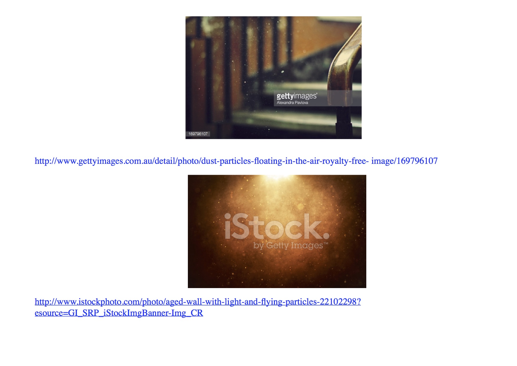
Video
http://www.gettyimages.com.au/detail/video/dust-particles-studio-black-background-stock- footage/532053237
http://www.gettyimages.com.au/detail/video/particles-smoke-dust-stock-footage/173045452
http://www.gettyimages.com.au/detail/video/shot-of-dust-particles-catching-light-london-stock- video-footage/500108359
Progress Report for the Dynamic Simulation
of a Dust Effect
This effect requires small particles of dust, that are visible in shafts of light, to be subtly floating in the air of a dusty room. The dust is an element, not the main focus and is reflecting the condition of the apartment, the environment.
I have looked at and used the client’s references and brief and have included further reference and research that I have found.
Dust Particles Dark Room Ray of Light – Royalty Free Footage. This is my preferred one, I like the flow, rate, speed, size and how they change with the change of light.
We are familiar with dust, a generic term used for minute solid particles. They are typically less than 500 microns in diameter with various textures and sizes from microscopic particles to grains of sand and consisting of soil, pollen, hairs, skin, meteor dust and many other materials from our environment.
My research included finding some of the qualities of dust particles and how they move. The are suspended in the atmosphere moving around the room at the speed and direction of the air current, exhibiting constant and random motion, like experiencing a buoyant force or Brownian motion.
These forces can prevent the particles from falling, lifting them higher, keeping them aloft for longer with the random motion being propelled by both collisions with invisible air particles and the dust particles themselves.
The dynamic nature of dust particles suspended in a beam of light is influenced by the chaining pressure, temperature and humidity or kinetic energy in the volume they occupy.
We are seeing a mix of mass motion of the particles with different density, size, weight and mass at different distances from our eyes that are being affected by the light.
Rays of light can be seen when light passes through dusty air, are we seeing the particles or are we seeing the light scattered by them. The particles are small, is it flashes of scattered light from the motion of the dust particles?
House dust is reflecting different wavelengths of light by many particles, the random scattering of light rather than reflected light. They are not individually reflecting a lot of colour information to our eyes giving a whitish or grey appearance. Even a huge pile of dust appears grey from the diffused light, especially the diffraction of light around the edges.
To create the visual qualities of dust, as explained in the client’s brief and from my research, I have used Maya’s, dynamic, nParticle system to generate this effect. I had made the dust movements smaller and subtler than the reference which can be adjusted with the field attributes that move the particles.
We started with the environment and initial particle set up in class, using a poly shape representing the space for the dust particles. Starting with a Resolution of 20 (number used to fill), Close Packing (how they align in the space) on, Double Walled (if double walled geo) off, Nucleus Space Scale to 0.01 (gravity is appropriately applied), Conserve set to 0.98, (the ability to conserve energy) and the objects in the environment are passive colliders.
Enable ignore wind and solver gravity enabled, the particles are not using the gravity and wind of the nucleus, Self Collide is on.
To achieve randomness I have used two particle systems, adjusting the attributes slightly differently on each one A then B.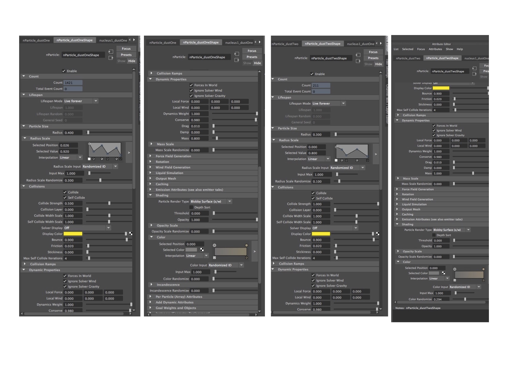
Particle size : radius to 0.4 and 0.3
Radius Scale : Randomise to 0.3 and 0.1, with Radius Scale Input to Randomized ID because creating different sizes and not changing over the duration of the age of the particle. Adjusted the widget with random values. Had fun with lots of different sizes.
Collisions: Collide Strength (>1 dampened the full collusion and preset
Dynamic Properties: Mass (density, nucleus gravity greater than 0) to 0.8 and 5.0, Dynamic Weight (scales the effect of fields)0.8 and preset
Shading: Colour to Randomised ID and used the widget with random values.
Starting with a Uniform and Turbulence Field for the velocity or speed and weight or mass to control the particle’s movement.

A Uniform Field is like gravity, using a lower magnitude (strength) and attenuation (how much the strength diminishes with distance), direction of -1 in Y to look more like floating, with no attenuation they fell straight down.
The Turbulence Field is giving the particles a more random motion. With the attenuation too high there are lines, too low they are running wild, also do not want them running up to the ceiling, into the corners or running for their lives. Higher values in the Frequency will give me more irregularities in the motion.
These fields are connected to both particle systems and I have added an Air Field, only connecting to nParticle_dustOne adding more randomness. Being set for the wind default which are working having increased the speed from 0.5 to 0.7 which can easily be adjusted later. The Speed attribute when set to 1 will matched the speed set in the magnitude, the velocity almost instantaneously.
In class we started working on the lighting, looked at the volumetric and cast volumetric shadows option and its effect with intensity. It was causing unnaturally looking shadows and colours from the shot camera.
Created an area light to illuminate the particles, breaking the light linking to the room, was too strong. Turned down the anisotropy value to 0.8 on the aiVolume node in the Hypershade. also considered lowering the light decay and turned on emit diffuse to soften the edges of the particles.
On the spot light I have changed the shadow colour to looks like some light is coming from the front even thought the area light is only lighting the particles.
For rendering we started looking at shaders, the surface shader did not work (it is a flat-coloured surface), used an aiStandard shader. Turned off visible in reflections and visible in refractions. Set the ray depth to zero. Set Initial State. Turned off diffuse light, making a direct illuminator, not sure about this as dust is very diffuse and considering the shader diffuse values, need to think about this.
Lighting and rendering needs more thought and could consider the use of bokeh, volumetric scattering and fog shader.
I like how the particles have a feeling of depth in the room, a resistance to the environment, with the appearance of lingering, randomly floating or weightlessness.
It can be as technical as we like, at the end of the day we have an instinct for how dust looks and feels, the aesthetics. Is it conveying the feeling and emotion? Is it right for the scene? Is it what we want to tell the audience? The amount of dust and values such as density, scale and randomness can be adjusted for the final feeling that will want to be expressed.
Additional reference that I sourced:
Stills
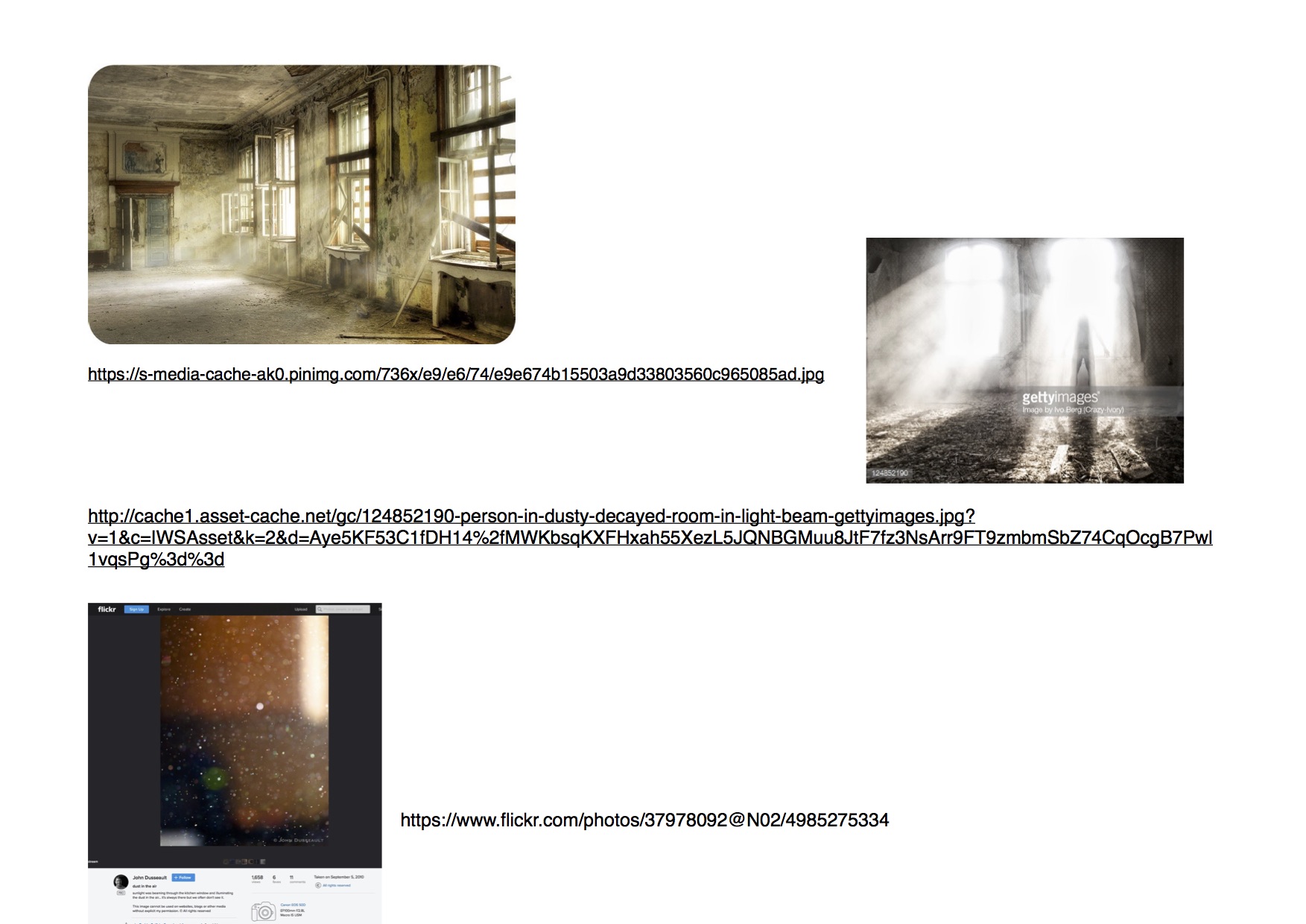
https://s-media-cache-ak0.pinimg.com/736x/e9/e6/74/e9e674b15503a9d33803560c965085ad.jpg
https://www.flickr.com/photos/37978092@N02/4985275334
Video
DYNAMICS 001 BEAM

make larger to see the toon particles on the side of the beam
I liked the idea of using Toons when we did it in class and wanted to see what this might do. The though is to shape the cylinder along the lines of when the spacecraft doors open and the beans would spread out at the same time then falling to the ground. I have done a rough shaped of the cylinder as a test and used the polyDisc to move to the ground with the particles emitting as the disc animates over the cylinder. It is bit hard to see the few particles in this slide, I like the way the particles are creating another layer of texture around and out side the beam. Again I have kept the settings basic to see how it might look.
-

- vertical s shape ep curve – points
-

- verticals shape ep curve streaks
-

- different direction
-

- circle ep curve from cylinder
Emitting particles from an ep curve with Directional emitting from the edit points, direction Y -1 and Emission Speed Attributes, speed 10. I then looked at doing a circular curve at the base of the cylinder geometry (my standby space craft) and controlling the number of beams from the curve’s edit points.

both ep curves

goaled particles
Here I set the streaks that are being emitted from the ep curves edit points as the lead particles and created a follow omni emitter, with the MultiPoint option in Particle Render Type, rate of 100. Turned off collide on the follow particles and can adjust the width with Multi Radius under Shading.
-

- beams not goaled to geometry
-

- goaled to geometry
-

- changing the shape of the geo changes where the beams go
-

- animating the geometry and the beams follow have also created the circular motion
Using a single omni emitter set in the cylinder geometry, 10 particles/second, emission speed 1 the beams were directed to the edge loops on the torus. Particle: Live forever, conserve 9.5, dray 0, Particle Render Type streaks, Line Width 10, Tail Size 1. Under Goal Weight and Objects the Goal Smoothness and TorusShape1 gives me options to create either the straight beams or the circular motions. Goal Smoothness at 3.6 and TorusShape1 at 0.15 gives me a broken line and it is more flowing and circular motion. Using a volume emitter, Torus gave me access to the Volume Sweep and Section Radius.
-

- increasing tail size
-

- increasing the rate (particles/sec)
At this point I would like to look at how I might be able to create a more solid, semi-transparent shapes for both the main tractor beam and to add variety to the area around the beam. The other thought is how to create texture with a variety of size, opacity and density.
testComp Video: password – dynamicsFirstTest108
Refining the ideas:
Starting to working on the idea of sparkles when the space ship door opens to send out the tractor beam to pick up the character.

Using nParticles I started with Goal Weights to take on the form of the polyDisk and was not able to get it to work how I wanted. I had done some tests using a curve and this did not give me the sense that the cap was full of sparkling type movements. Then I looked at using emit from Surface for the particles and did some tests to see how the emitter worked and how the particles could look. I was attempting to get a random, sparkling effect across the opening before the tractor beam comes out. Initially the particles were still falling from the geometry, turned off the Ignore Solver Wind and Geometry and then adjusted the values on the emitter. I chose points, emit from surface so they would cover the surface and not be from the geo’s vertex.
Adjusting the values after awhile I realised the normals were facing the wrong way, I rotated the polyDisk though could have changed the normals direction. I put the Speed to 0.5, Speed Random to 1, Tangent Speed (not just emitting in the direction of the normal) 0.5, Normal Speed (controls the magnitude or strength of the velocity) 0.5. Using both the speed and normal speed to give some depth with the particles not completely flat on the surface. Then the tangent speed and speed random added some randomness to the emission. Particles do not understand how to behave in the atmosphere how we are used to experiencing our world and all these attributes and values need to be assigned. At the moment the rate is 800 and I am happy with how that is covering the surface. I have put a max distance of 0.3, the min and max distance control how far from the emitter the particles are created, giving some depth to the surface particles.

I need to control when the particles stop so they are not live and continue to be emitted when the space craft moves off. On the ParticleShape node I have used Random Range for the LifeSpan setting it to a LifeSpan of 5, Random 5 and General Seed to 2. The idea is to add to the randomness created by having the particles live random amounts of time with the General Seed randomising how the lifespan random is distributed amongst the particles.
Adding to this and creating a more sparkling effect I have added a per particle colour attribute and used a ramp to vary the colour during the life of the particle. The point size is 3, too large made it look like a solid coloured slab. This is working for the initial idea of sparkling colour appearing when the space craft hovers before sending out the tractor beam and also while the tractor beam is operational.
Now I will look at setting up the beam and see how they work together.
-

- surface emitter from cylinder using texture to control the emissions
-

- toon shape to emit the circular particles
I have created a tapered cylinder for the tractor beam and animated the black and white texture values to control the surface emissions. The grey scale ramp has been mapped into the Texture Rate attribute of the emitter. It uses the black (0) value, no particles emitted and white (1) values with the totally rate set on the emitter to control when and where the particles are emitted. As it is a multiplier the emission rate is multiplied by the colour value in ramp with the grey values adding more variety and control. I like the option to be able to change the geometry’s shape, and animate the toon geometry that was created in order to make adjustments to the particles.
Using a V ramp, right hand side of the ramp is the top of the cylinder and interpolation set to smooth which is a bell curve blending quickly to the next colour. This could be adjusted with none being more like bands. There is a Noise attribute giving offsets from the U and V directions which I have not used at this stage. I have used the toon idea from my experiments to add variety outside the beam. There were originally two distinct shapes and I have scaled the toon geometry to be closer to the other geo shape. I also liked the idea I worked on with the particles being goaled to an animated torus shape that was looking around for the character. I will add these and see how they work together. Have not use gravity or wind attributed on the nParticle to move the particles.
-

- surface emitter
-

- directional emitter
-

- omni emitter
Here I am looking at creating the beam of light using a CV curve as a motion path for the sphere. I have chosen cloud for the particle type and looking at what type of emitter. I think it is going to be a directional on and will look at keyframing the direction to change from the down to the up movement. With directional I have the direction x, y, z available on the emitter but the particles are emitting from the vertex.
-

- sphere, emitting particles from vertex
-

- cube, animating along the curve
For the line shape beams I was decided to go with motion tracking instead of goal weights to an animated shape. I had trouble working out how to have the CV curve positions so it looked like the the shape moving along the curve was in the right place. Also how to have the beams go down and then come back up, hello, put a u turn in the curve, why does it need to stop at the bottom. I have a working cylinder set up between the space craft opening and the character and when making the curve I eventually worked out to snapped the points to it to position curve line shape look thus looking like it belongs as part of the sparkling beam. It is a Directional emitter with 1 in the y direction, life span is constant at 10, particle Radius at 10 and the Radius Scale tapers off for the tail.
Under Shading the Opacity ramp has been adjusted from about half way at the beginning to full a third of the way and tapering to zero at the end. Now how do I control when the particles start and finish. Finally I worked it out, I can set key frames for the U Value on the motion path to control when the movement starts and stops, will now look at adjusting the speed along the motion path like when it leaves the bottom and the twisting. I am still having problems working out why and controlling when the particles turn on the motion path. I am thinking it might have something to do with the direction of x, y, z in world, local or object space when I set up the motion path. Still working on that.
-

- particles staying too long
-

- rate keyed at 0 to stop particles, was looking at making collide with some geometry
-

- beams still crossing the geometry
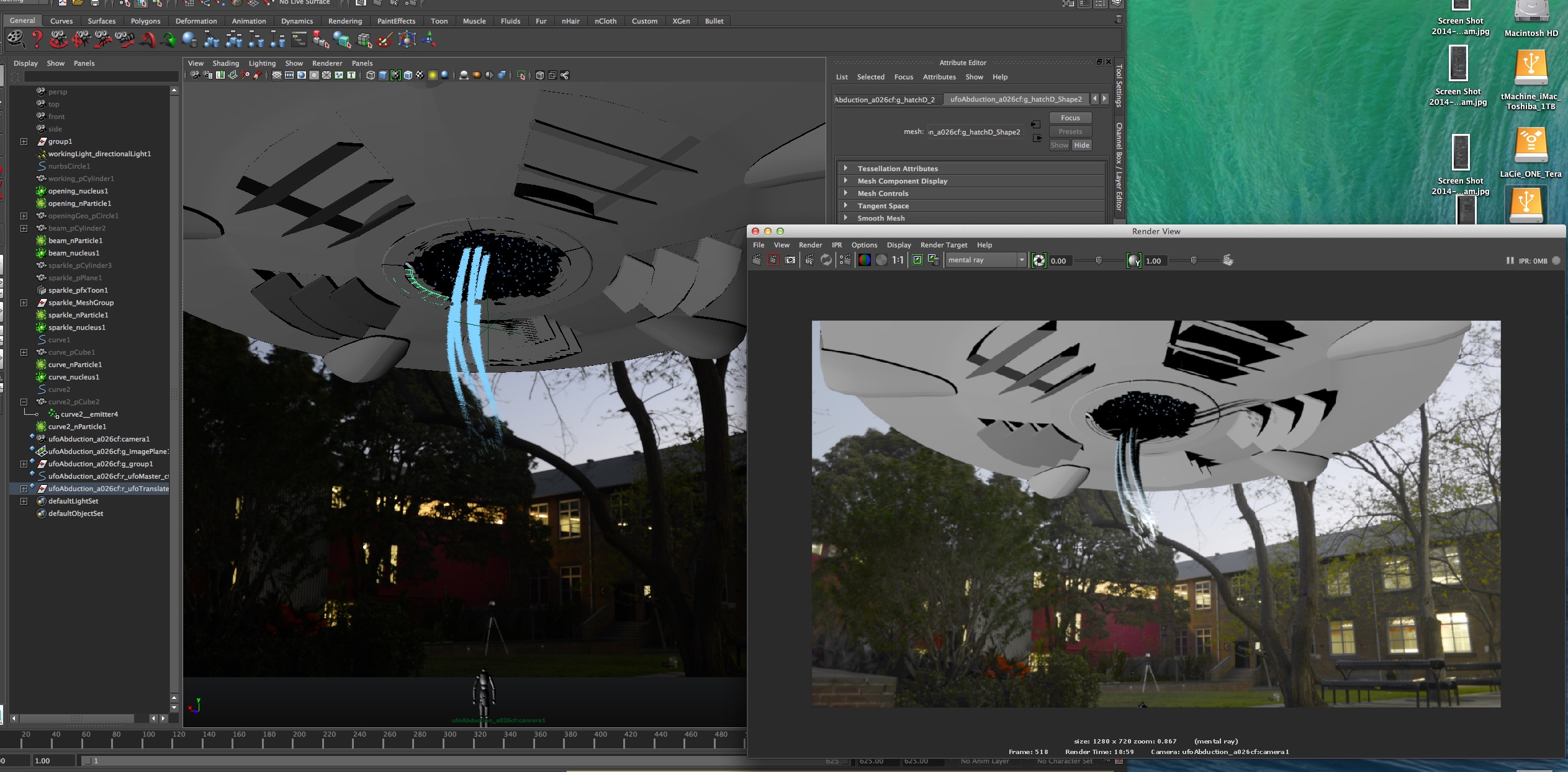
need to do some work on the colours, opacity, transparency and alpha
I need to look at a few things like adding depth sort, including more random attributes such as particle size (link radius scale age to randomised ID p13), fields, maybe a Newton field, having particles collide with each other using force fields or particles emitting particles. I’m not sure about the horizontal streaks in the long line particles beams. I’d like to work more on creating bursts of particles by maybe key framing the rate or key frame goal weight and goal smoothness.
Rendering
Chris, I need help with the rendering side of this and have not worked out about using the back plate and compositing in Nuke. I rendered out the whole scene, thanks for the heads up about leaving a week for rendering. I stopped working on the particles on Wednesday of the second week of the break and started rendering. The first render went from Wednesday evening and by the week-end it was still going so I stopped and rethought it all. The up side of this is that I re-read the class notes and found this very helpful. It was suggested I change the render setting quality from 1 to .25 which I did and picked up where the first render had stopped. I realise that I needed to cache the particles when splitting up the render like this and due to being a bit stressed about time and not really feeling like the particles were looking very good I wanted to at least have a render to hand in. I have supplied a playblast and I think there is too big a difference between this and the render. There is a problem with the colour of the particles and I need to work on the transparency/opacity issue. For some reason I thought I did not need a PSI node for nParticles and not sure if this is the issue, I need to look at it.
The other thing that I would like to have done more of is go back to your video about the brief while I was doing the particles. I looked at it again after the render and feel there are a few things that could be worked on and added to the particles. This would look at some breaking up of the particles with differences in the variety in the colour, texture, rate, opacity and size; like the ribbon effect you mentioned and some finer detail for contrast and depth. Maybe when I brought the two cylinder geometry shapes closer together I could move them apart again and work on the differences. I like the sparkles, it does look a bit different but at the expense of probably not having enough of the cloud and vapour like appearance adding to the sense of motion. I like how the dots move down and the graduation as they move give gives a sense of motion, again maybe some more variance. I changed the circular ring motion on one of the cylinder shapes for a more bended movement as they move and thinking about it the circular motion might have created a great sense of movement, randomness and contrast. I have not managed to build the wispy trails with some scatter disappating in the atmosphere that you spoke about or the smoke, vapour or mist feeling. The line type beam particles also need more variance and changes in intensity and maybe this is where I could have a stronger sense of changes in colour like when you spoke about the heat intensity of the beam. Maybe a couple of these longer beams could be the ones to introduce the wispy tails and the cylinder shapes have more of the cloud or vapour effect.
Assessment 1 (b): Process Diary – week 15
Taking the tractor beam simulation from part (a) in week 9 with feedback and further research develop and take the dynamics further
Some of the problems I had working towards the week 9 assessment have been sorted out including the position of the ufo camera in my scene. The focal length has now been set to 27.0. I was not able to get the perspective camera happening which caused a bit of stress. There is also the option to reset cameras by selecting it > look through the camera > view > default view or dragging the perspective camera into the viewport.
General Feedback
– how does the tractor beam work, the mechanics of it and how the elements work together when combined. Why are the particles doing what they are doing
Tractor beams use light to move objects, like a blast of water. The light beams exerts a tiny force of light, a forward push when it hits something or it can also pull.
This force comes about because the electric and magnetic fields in the light polarize the material in the object, and the polarized object can then reduce its energy by moving to where the light is most intense.
By adjusting the material properties of the object and the polarizations and synchronization of the individual light waves in the beam, physicists can make the object radiate more light forward along the beam than backward toward its source. The radiated light then acts like a reverse thruster, overcoming the already-reduced forward push of the beam and driving the object back toward its source.
Not Pulling Your Leg: Tractor Beams May Be Possible
…it draws an object toward it without making physical contact. “By shaping a beam of energy so that it goes around an object in some way, hitting it in the back, it’s possible to then pull the object instead of push it.”
An Advance in Tractor-Beam Technology – July 30, 2014

This NASA video describes three ways used to draw in objects and together with my reading about how tractor beams work I’m going to look at the Bessel Beam which uses concentric rings of light to snag the matter. This could possible work with the suggested idea of the circles.
The other two were optical tweezers which is a pair of spinning beams pulling matter into the dark corridor between the beams and optical solenoid which uses the laziers spirialing intensity peaks to pull particles back along the length of the beam.
Tractor Beams May Actually Work: NASA Studying 3 Methods

Bessel beam spreading at a length of one-quarter of a millimeter in a scattering medium. Source: Bio- und Nano-Photonik/IMTEK
Researchers Achieve Better Illumination of Biological Samples – Publication in Nature Communications
Pushing and pulling using polarized light
Optical Tractor Beam Sorts Tiny Particles
– what parts of the reference image is relevant, break it down and think about what I am attempting to design. Talk about it and create my own concept art to help make my imagination a reality
– what is it about existing tractor beams that would make the audience feel comfortable
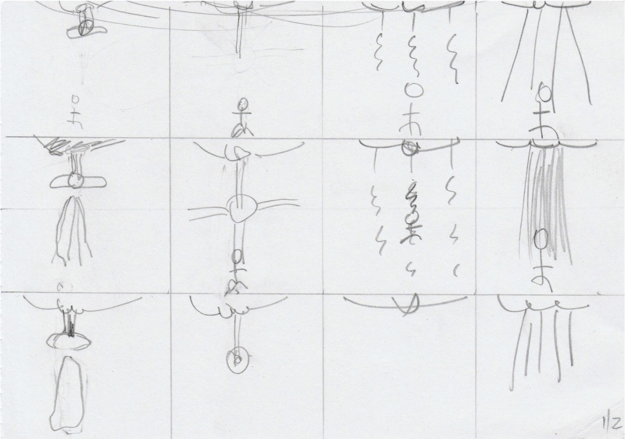
some thumbnail drawings exploring different ways the tractor beam might be able to work

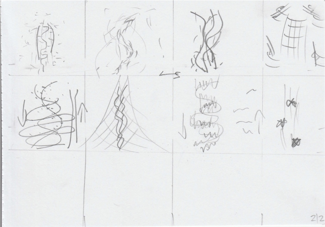
When I first looked at the tractor beam I initially focused on more traditional ideas, then I started exploring alternative images while considering the tractor beam being a non-threatening experience. I went back to my drawings and looked for more references.
The Gardens by the Bay in Singapore light show images reflect happy, fun time and are something different.

– add something to create extra movement, possible lines that run down the outside of the outer cone then spray fine misty type particles, they could be thin circles or tubes that move down the cone from the ufo
From these different drawings I continued focusing on the sparking idea as this reminds me of happy times like Christmas and party time lights. I’m considering the ideas of the traditional tractor beams and how they work using circles of light together with the sparkles for particles. With the spiral, tendril not working and deleting the idea as suggested I’m now focusing on how to create movement with the moving circles and how this will work with the sparkles.
– consider these attributes: Mass on Particles – which can give subtle variety of movement, Conserve – can add further variety of movement with small changes having big effects, Oversamples – in the Solvers Menu and may help with gaps in the particles and will make the simulation slower, Lifespan, varying it on the particles to add variance to movement and form, Fields – could make more use of this in having the particles moving, Depth Sort – if not using show that it has been considered, also consider Lighting and Colour Accum etc.
I have used the ramp in Mass Scale for two of the particle systems to vary the mass which determines the density or the weight of the nParticle, a lower Mass value and they will mover faster.
I have left conserve at 1 which influences the particle object’s velocity from frame to frame with 1 they will not lose any energy.
The oversamples are at the default value. Specifies the number of sub-steps for each frame of your dynamics simulation. A value of 1 sets no oversampling. A value of greater than 1 causes Maya to oversample your dynamics simulations by the specified value. You can use any arbitrary value for Over Samples, as long as it is a positive integer. You can often fix excessive dynamics behavior by increasing the oversampling of your dynamic calculations. Increasing oversampling slows down playback but increases the stability of your dynamics.
The Lifespan for two of the opening of the UFO and the inner core are Random Range to add to the sparkling effect and the outer core beam has a Constant value of 0.1 so it looks more like the moving circle and the particles are more attached to the shape.
For the Fields I have introduced a Gravity Field for the inner core beam as I found it slightly changed the shape of the points in a random way, not so round. The field does not have a large impact on the actual movement as it is a surface emitter, I like the subtle change it has caused in the particle shape and I think it helps with the flickering.
I have turned on Depth Sort for rendering which sorts the particles based on their depth from the camera, Colour Accum which allows overlapping particles to influence the colour of each other.
– shadows for the mannequin for rendering, possibly light from the tractor beam to light the mannequin and talk about it. The mannequin is reacting to the light of the tractor beam and feels like it is inside it.
I have created a shadow pass for the mannequin to be used for the Nuke compile. For the tractor beam a glow on the beam in Nuke works much better than I would be able to create in Maya.
– reflections and ambient light, are the particles visible in the UFO
I did not like the idea of the particles being visible inside the UFO, as the particle’s purpose is to focus on the mannequin and to relate to it being lifted up into the UFO. Actually I think you might be speaking about seeing the particles on the surface of the ufo. This would possibly look great though have not gone down this path at this stage.
Things for me to work on
– explain more what parts of my reference images are relevant and what I would like to incorporate
While I was looking through references and drawing the shapes I started to notice some of the qualities regularly used as part of tractor beams such as lines and swirling shapes. Parts of the images had sparking qualities and as I have mentioned in the general feedback I began to focus more on this area of possibilities.
– talk about when using certain techniques I am able to create a simulation that looks like the images gathered
After using several different render types each time it came back to points when looking for ways to make them sparkle.
For the particles at the opening of the UFO’s the geometry emitting particles is now positioned at the UFO’s opening thanks to the perspective view, called opening in the outliner. They make the opening more obvious when introducing the particles here, revealing them as the hatch door opens. It is a surface emitter defining this shape without much movement from the surface. TheBasic Emission Speed Attributes of Speed 1, Speed Random 1, Tangent Speed 0.5 and Normal Speed of 0.5. This worked better as a polyDisc instead of a curve for the opening shape to be able to fill the space with particles.
To create some interest with contrast and movement I have put black and white values into the emitters Texture Rate and a colour ramp in the particle’s RGB PP. I have added more colours and lightened them to fit in more with the colours of the other particles while leaving them darker than the others. This works for keeping them the same but different from the other particles and adds to the perspective depth between the particles and area of focus. Radius is 0.2 to keep them small with 0.5 for Radius Scale Randomize and included some opacity with the Opacity Scale.
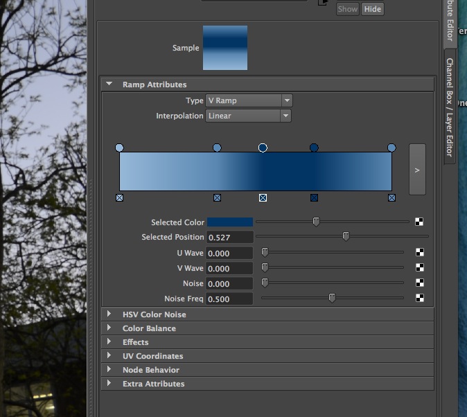
less variety in the colour and darker blues

more detailed colour ramp and lighter colours
– more detail in the movement, more particles the particle count will help add detail, the tractor beam is hard to see and needs to feel more like a light source
There are two other emitters, the first one is a surface emitter called innerCone and the second is a toon emitter acting as another tractor beam or outerCone.

Working on the inner cone first, I’ve make this smaller to see the difference between the two beams more clearly and build some variety. The geometry is tapered more from the UFO opening to the mannequin, making it not so symmetrical, a surface emitter with Particle Render Type as Points.
Staying with the sparkles, firstly increasing the number of particles, the particle count to 30000 making a more defined shape and a speed of 0 for them to stick to the surface. There is not enough change happening in the position of the particles, Radius is 0.2, Radius Scale Randomize is 0.2, using the ramp on Mass Scale and Opacity. It was still looking too solid and no movement in the shape.
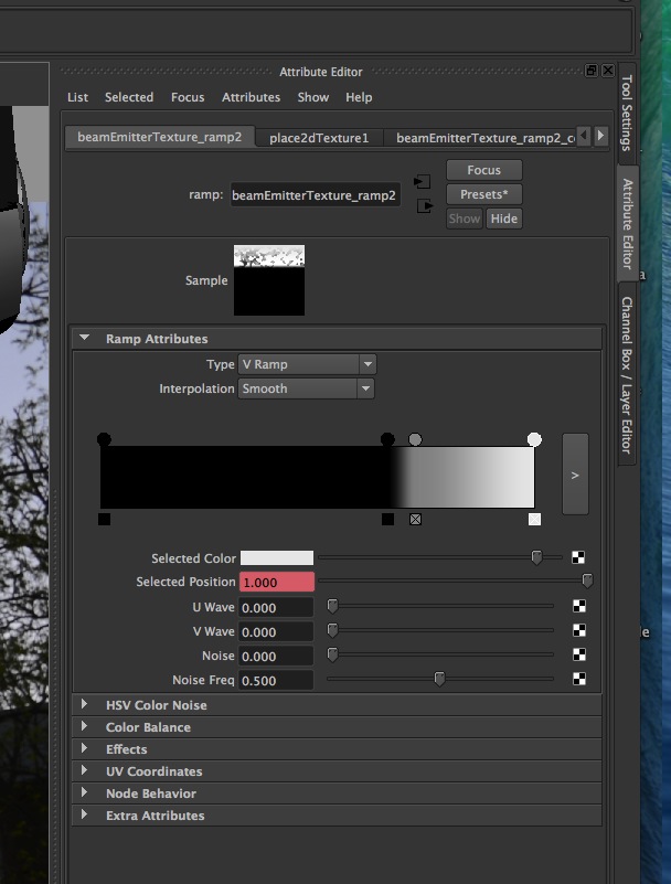
Going back to the Texture Ramp, on the emitter, to see how I can introduce and control more randomness with the particle placement and how the shape is appearing has been interesting. I looked at what might work by adding more black and white points on the ramp and adjusting the gradient with these values. Emitting particles from the white areas and the grey scale is a multiplier for the rate set on the emitter. The timing of the particle being emitted now changes more often and more in timing with the idea of sparkles and the black areas are creating some empty areas which I like.

I have also mapped a fractal into the white and black colour selection of the ramp to add more randomness and sparking. This is not working how I had imagined and totally taking away from the down movement and the black and white controlling the particle emission was lost. I took the fractal out of the black and left it in the white adjusting the fractal values to get more control. It is not only the sparkles that has started to happen in areas it is more like the beam is pulsing on and off as it goes down to the mannequin.

Animating the position of the points on the ramp, creating different black and white gradients over the time gave some lovely changes to the particles that were being created. This together with the fractal has added a gentle pulsing movement and the random placement of the particles leaves spaces along the shape. I’ve added a gravity field to the innerCore and it gives the points some different shapes.

changed the shape again, adjusted the opacity, lightened and varied the colour
– likes the sense of an outer cone to the tractor beam, add something to create extra movement, possible lines that run down the outside of the outer cone then spray fine misty type particles, they could be thin circles or tubes that move down the cone from the ufo
– likes the idea with the cone acting like a ring that moves along the surface of the outer cone to emit particles, revisit what I did with toons in my reference
The outerCone emitter, is MultiStreaks, is a combination of Streak and MultiPoint render types and it displays multiple points with tails for each moving particle. The faster the particles move, the longer the tails. The inner Cone emitter is points, displays particles as points, although they both look like points I think it gives a subtle difference.
Increasing the particle numbers, lifespan, geometry shape and how it is sitting over the top of the innerCone and creating some rings.
The colour is changing from white to blue as it moves along the beam. Possibly giving the illusion the light’s heat changing and the beam travels. The colour ramp has been reversed and the Input to Normalized Age.
On the emitter I have adjusted the Speed and Tangent Speed to give some direction as the particles are emitted. Depth sort is on, it is where the particles occlude each other, the render is working out which particles are in from of other particles with the render only displaying the particles it can see.

version one with 500000 particles
The start time is 330 and the particle numbers have been increased to 50000.00 and a longer life span. Now I am not sure about the streaks, have put it back to points and the Lifespan from Random Range back to Constant with a Lifespan of 1. The particles are looking more like they belong with the others. I still have a problem with it appearing a bit flat and not a shape for the mannequin to be pulled up in. I love the circles that are starting to give the beam a sense of movement and some shape. The gap between the the inner and outer core implies that there are two beams and wonder if they were closer if they would get lost with each other. Also wondering how similar or different the colours need to be.
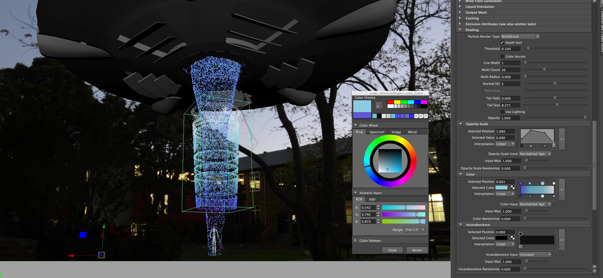
For this outer tractor beam I am using the Toon option which is part of the rendering menu set. Particles will be emitted from the collision point of two objects where Intersecting Lines are enabled. This intersecting line is converted to geometry, pfxToon1 node. The Mesh now Emits Particles from object and is a Surface Emitter.

Chatting with Chris there is another world out there with want is possible when looking at how to make this a repeating smaller circle that is travelling along the tractor beam shape.
Instead of only animating the movement once, making the animation much faster and repeating it gives the effect that many circles of light are moving down quickly instead of a beam that is streaming down creating longer shapes. In the Graph Editor > Curves > Cycle with Offset and View > Infinity.
Line Width can be adjusted on the pfxToon1 Node and being set to 5. The emission rate is now 50000 with a start time at 330 frames and the rate is keyframed to 0 later in the simulation to stop the particles being emitted at the end of the tractor beam sequence.
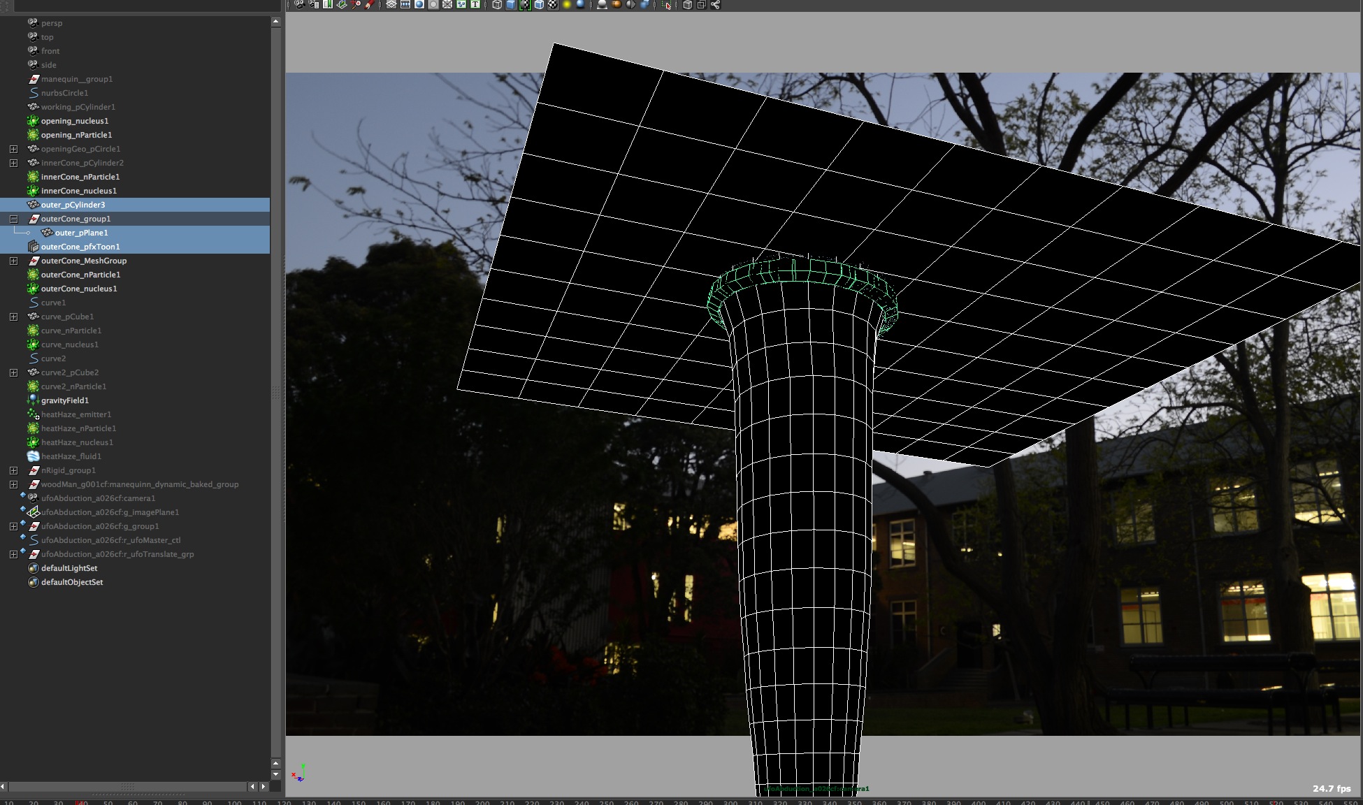
thought it was great when I say the pfxToon1 geo being translated and scaled
Other options Chris looked at were Duplicate Special for the polyPlane > Input graph option to copy the animation over but this did not seem to work out with the animation in the Graph Editor. Also linking the polyPlane to the correct Nucleus, creating an emitter and selecting a nucleus, using nSolver > assign Solver to Particle, changing the Line Width, connecting emitters and particles.
Reducing the speed (how quickly they move from the emitter) attribute to 0 did not keep the particles on the surface to attempt to give the look like the particles were sticking and keeping the shape. Also the Normal Speed which controls the Magnitude did not appear to be working how I would have thought.
The Key Visibility option for the outerCone_MeshGroup did not change how the particles were emitted. The Lifespan is constant and changed from 4 to 0.1, Radius Scale’s graph goes from 1 to 0, Opacity scale a round curve from 1 to 0, and the colour is similar to the existing beams and Motion Blur enabled.

can you see that light circle around the innerCore particles?
Chris, thanks working through this. After having another look at it I like the slightly odd shape of the inner cone as I think it works ok with the random sparkles. I was really excited when I saw them in Nuke and how the background is showing through the spaces in the particles. It brought them alive and gave them more depth. Really shows how I need to see them on the background.
The outer line is sparkling to fit in and having them move faster with a smaller height has a much bigger impact on the overall movement that is happening. It does not get lost with the other particles and takes your attention there. At first I did not like how you could not completly see the mannequin being lifted, now it feels like there is a bit of mystery. Is that the mannequin you can see moving inside the particles and when the beam goes back into the ufo the mannequin has gone, must have been taken inside the ufo.
I have left the colour lighter, helps create some depth, the space between the beams is showing off the movement and is looking much better than having the longer trail of particles coming down the shape. It is not so much of a blob of particles and gives more interest.
– tendrils are not working, not connecting to the outer cone
This is a geometry moving along a curve motion path with a keyed start time frame in the U Value and particles being emitted from the geo’s vertex points. When I thought the main tractor beams did not have enough depth or perspective I did go back to putting these inside the core beams and having them much finer. They are definitely gone now and with the circles working the way they are this is a much better way of solving this.
– check lifespan set to 1 and random range set to 1 on one
fixed
– remove the ambient light
done
There are some general things I wanted to address including the attributes mentioned in the general feedback.
At the beginning I did not think through some things such as nParticles having different nucleus meaning the particles are not able to collide. I could have used the nCache more which writes the particles to the hard drive in the Image folder of the project. This positions the particle in space for each frame and when using the timeline Maya is not reading other frames to position the particles for each frame on the timeline.
Initially I did not want too many because what happens is when the UFO doors open it is full of particles and I prefer that it looks like it is building up, increasing with the sparkling on and off before the tractor beams start. I’ve increased the number of particles being emitted (sets the average rate at which particles are emitted per second), added more variety to the radius scale for subtile randomness, changed to Normalized Age (the per-particle attribute values are mapped within the range of the nParticle object’s lifespan) and changed Lifespan Mode from constant to Random Range (identifies a range of random variation for the lifespan of each particle). Looking at Mass Scale ramp, it is a bit hard to tell how much this is changing the particles as they are not travelling very far, maybe very subtile and adding to the variety, have also set this to Normalized Age. Set the Mass Scale Randomize to 0.5 (Sets a random multiplier for the per-particle attribute values). Turned on Depth Sort and have left the Opacity Scale at Linear, I think this will add to the sparkling effect and input to Normalized Age.
Now to sort out the colour, I have used the Per Particle (Array) Attributes which lets you set the value of the attribute individually for each particle of the object. I am going back to the reference to see what I can do here. I’ve taken out some of the black and introduced some more colour shading.
Rendering
Now doing my rendering in Hardware Rendering, not Software or Mental Ray. Turn off Colour Management (sRGB), padding 4, name.#.ext, render camera, use an image format that supports an alpha channel, select Alpha under the Renderable Camera, Number of Samples which 1 being a hard edge (bit like anti aliasing with more samples giving a softer edge) used 9, enable Geo Mask, possibly Motion Blur, Production Quality, Motion Blur and Frame BufferRGBA: 16-bit float per channel. Do not need the option box for Batch Render as the Render Settings does this.

rendering from week 9
with the changed colours the render looks totally washed out
One of the problems was with rendering the particle’s colour, I’ve stopped using Mental Ray and staying with Hardware Rendering. Now that has sorted my colours, they are consistent and I am more confident when choosing colours.
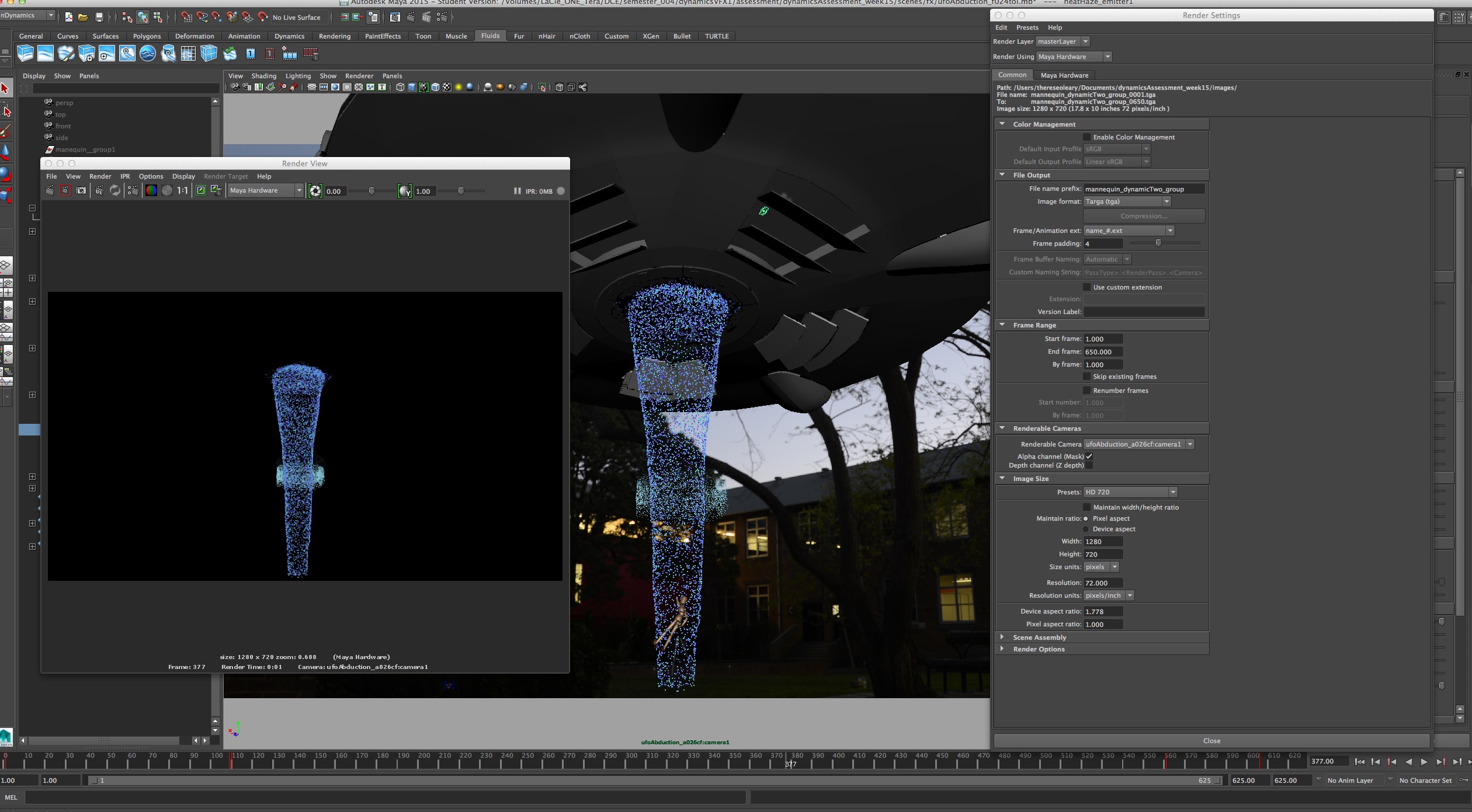
now I have renders
Can create a cache, nCache > create new cache and make sure the project is set and the cache goes to the projects Images folder.
Render > Batch Render and do not use option box because the setting have been set up in the Render Settings, Maya Hardware options.
In Mental Ray it converts particles to geometry. The streaks tails need a transparency on the shader to fade the particles from head to tail. There is a connection with opacity, transparency and the alpha channel.
For the Toon have the Render Stats > Primary Visibility> off.
http://help.autodesk.com/view/MAYAUL/2015/ENU/?guid=Particles__Create_Emitter
http://download.autodesk.com/global/docs/maya2014/en_us/
Baking Dynamics
I had problems with the scale of the dynamic mannequin. With Chris’s suggestions the solution turned out to be to bake the simulation. I did this by selecting the translate and rotation values in the channel box. This was not enough, when I scaled the mannequin the constraints were still there, full size and only some of the geometry was scaled. I needed to select all the geometry when baking and then deleted the constraints from the outliner and the scale to 0.5 worked fine. When I was scaling the geometry without baking the simulation the constraints were not scaling with the geometry.

Baking converts the dynamic induced animation to keyframed animation and the animation curves can then be tweaked and manipulated like all other animation curves. It is like caching particles so when played it is already keyed and if the dynamics break all the keyframes are there.
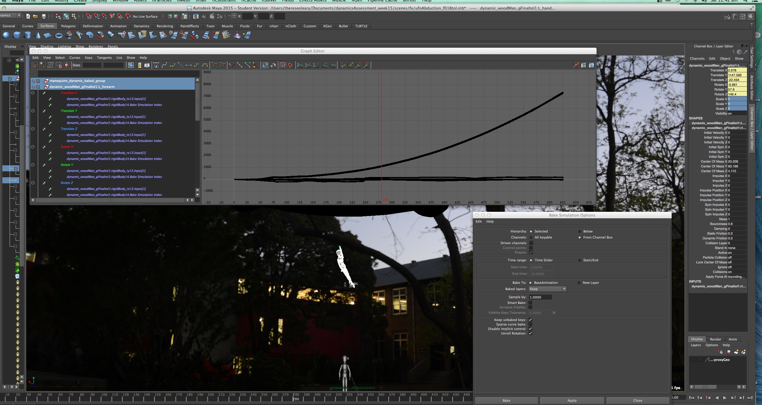
Remember when importing if it has been referenced then import from the Reference Editor > Right Click > File > Import Objects from Reference.

Heat Plume
Starting with nParticles like we did for the basic smoke trail in week 5, using a volume emitter, adjusting the volume emitter with a shape cube, scaling and positioning it inside one of the exhaust vents.
Keyframed the emission rate (particles/sec) on the emitter from 0 to 2000 and animated the emitter as the UFO moves away. Looking at the following attributes I set the Along Axis, Away from Central Axis, LifeSpan to Random Range (3, 2), Particle Size (3), Normalized Age, Depth Sort, enabled Ignore Solver Gravity, Threshold (0.5), Opacity (0.98), Directional Speed (10), and looked at collision friction and sticky.
Then I used the particleCloud shader and connected the PSI and reverse node to work out the opacity and transparency, rendering in Maya Software. Not happening. Below is a list of screen shots for what did not work, learnt a lot.
-

- test volume emitter shapes
-

- position of volume emitter
-

- test render in Maya Software with initial particles
-

- test render in Maya Mental Ray with initial particles
-

- thick cloud nParticle option with cloud s/w option for particle render type
-

- adjusting attributes
-

- adding the particleCloud shader
-

- adjusting attributes, animating the emitter and rate
-

- building the shading network for opacity and transparency
-

- added the psi and reverse nodes
The choice of the nDynamic particles of thick cloud was not the way to go. There are presets in the Maya nDynamic system with this option and it was difficult to know and control. There was no need to add another particleCloud shader and this doubled the problem so to speak and the default one was the one to go with.
After much checking with Chris it is back to the drawing board and going with what we did in class, week 7 for particle distortion and going through the notes. So here goes.
TAKE TWO, probably a few more than that – heat haze for the UFO
– create nParticles: points
– volume emitter shape: cube, scaled and positioned in one of the vents of the UFO.


– particle render type: blobby surface (s/w)
– added a blinn to the particles and made the colour black, transparency white, diffuse 0, reflectivity 0.
The Rate (particles/sec) has been keyframes from 0 to 250 to 1000 from the first frame to frame 139. Giving me a more of a sold look and a rippling surface.
Initially had trouble seeing the particles and the radius was too small, made 30. Lifespan is Random Range with 2 and 3. Depth Sort is on, Threshold is 0.5 allowing par tiles to merge with 0 having no merging.
Threshold: Determines the smoothness of the surface created by overlapping Blobby Surface nParticles. Threshold is based on the overall density of overlapping nParticles. Each nParticle has a density of 1 at its center, which then falls off to a value of 0 at the nParticle’s edge.
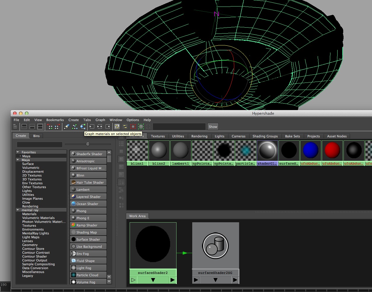
To see how this might look in Nuke I need to only render out the particles, everything gets turned off and a surface shader is used for the geometry of the UFO. There is a heat haze happening with the iDistort node and a Copy node to use the UV channels to apply greyscale values across the image. Have also added a blur node.
Now I want to apply this to all the vents of the UFO and also need to adjust the contrast values of my particles.

I am duplicating the emitter, then selecting the particles and under nParticles > Use Selected Emitter. I now have particles in each of the vents. I then parented the heatHaze emitters to the geometry and they will follow the UFO across the scene.
Another option was to create a locator, put the pivot point of the emitter on the locator with the emitter positioned at the vents and the locator parented to the spaceship. The animated keyframes for the rate can now be positioned for each of the emitter’s rates. I needed to make one keyframe on each emitter’s rate then was able to past the original keyframes and position them on the right frame.
Making the UFO geometry a passive collider means the heat plume particles will not affect it. In the make passive collider option box choose the solver related to the relevant particles.
When nParticles collide with passive collision objects, their behavior, speed, and direction change. Passive collision objects are not affected by collisions with other objects.
I am not sure about the reason for this as I rendered the particles on their own and used that in Nuke to create the heat haze effect with the iDistort node.
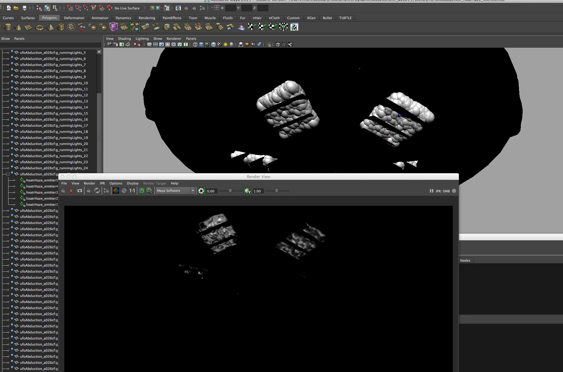
Re-rendering these particles and seeing how it basically works in Nuke against the back place I have heat haze distortion happening. Now I have this basic workflow set up I would like to do a lot more with the particle attributes such as having more control over the black and white values, the size and shape of the particles and how the move when the vents open and the UFO moves out of the scene. I will hopefully have time to come back and look at this. Chris thanks for your class notes they are amazingly helpful and help form some great class mates.
Would consider looking at:
Away From Center: Specifies the speed at which particles move away from the center point of cube or sphere volumes.
Along Axis: Specifies the speed at which particles move along the central axis of all volumes. The central axis is defined as positive-Y for cube and sphere volumes.
Directional Speed: Adds speed in the direction specified by the Direction XYZ attributes of all volume emitters.
Some things I was using previously that were not appropriate:
Self Collide: When on, particles generated by the nParticle object collide with each other. When off, these particles do not collide with each other. Which means I do not need to use the friction and stickiness.
Emission Overlap Pruning: Removes newly emitted nParticles before they appear in the simulation based how much they will overlap with existing nParticles. This value scales the collision radius used to determine overlap. A value of 1.0 it guarantees no self collisions with other particles on emission.
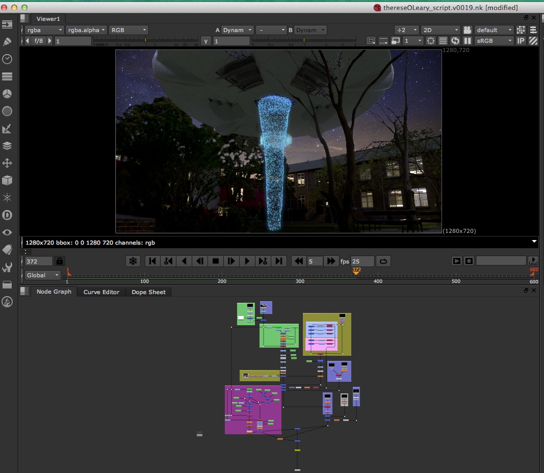
Notes – autodesk help files
Link to: Basic Emitter Attributes
MAYA HELP nParticles Shape Node link
The Brief References
My References
Stills:


More Recent References


From the Image Peace Tower web site


The stunning forest of giant metal trees at Gardens by the Bay, in Singapore is even more mesmerising at night. The structures light up in a rhapsody of colours to the sound of music that fills the entire park. It is ‘Supertrees’ that make this sound and light performance so impressive, towering above you at up to 50 metres tall. The show culmination when the trees seem to explode in a firework-like fashion.
-

- new york city tribute
-

- new york city tribute
Shutter Stock: underwater ocean waves ripple and flow with light rays:
Video – Youtube:
BULLET maya dynamic plug in
WEEKLY TASKS
I wish I had more time to spend on these, I’ve enjoyed when I have and looking forward to more when I can.
WEEK EIGHT – Rigid Bodies Exercises


I had a lot of fun with this. Did not get the cube to tumble, it is rotating in Y and I worked on having the ball hit the cube with the cube falling off the edge and the ball stopping before it rolled to the edge. I adjusted the initial velocity on the ball to hit the cube and adjusted the linear damping to stop the ball before rolling off.
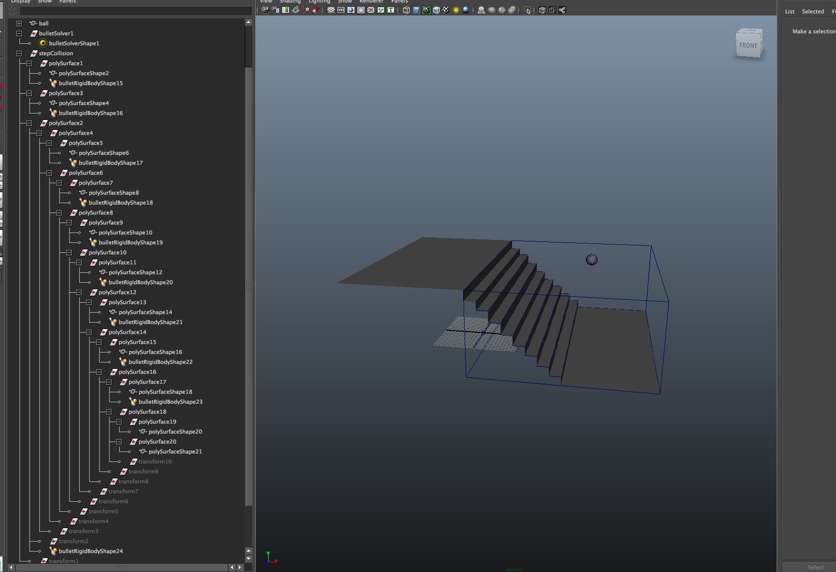
Still working on my ball rolling down the stairs. Have not been able to work out how Chris grouped and parented the geometry in the outliner and my ball is not rolling down the stairs. It is still rolling on the shape as thought it was a set to box in Collide Shape Type. I have redone the step geo and created passive rigid bodies a few times. Also adjusting the Collide Shape to Null and the restitution and initial velocity and not able to get this working. Not crying yet, will come back to it now going to look at Winnie the Pooh.


Hello Winnie the Pooh.
Pooh was exploding right from the start, for this to happen on impact
– in Initial State set to sleeping, collision type to Hull and the Wall Body Type on its RigidBodyShape to Static Body
For real world scale set the gravity to -980 on the solver
The cannonBall’s Rigid Body has an initial velocity of -500 in Z to have the ball land as in the screen shot above in the Initial Conditions. Then to land on the other side of the geo instead of falling straight down the Mass needs to be above 1000, I used 1500 giving the ball enough power to go through Pooh and land on the other side of the wall.
Pooh’s pieces are still falling through the ground and adjusting the rate at which the geo moves per frame worked this out. It was still falling through the ground at 120Hz and stopped at 240 Hz.


Using the glue on the Pieces Set Initial State gave me more control over when the pieces broke up on impact. The threshold value can be used to adjust how strong a force would be needy to break the object. The other issue with this is that the ball is no longer falling on the other side of the wall.
The ground needed some friction to help control the roll and movement of the broken piece, I set it to 0.5.
On the poohFractured_PiecesSetInitialState I set the Linear Damping to 0.3, Angular Damping to 1.0, Friction to 0.5 and Restitution to 0.5. How did they come up with this name ‘Restitution’, like English is short of suitable words? Glue is set to 70.
The red cannonBall has a mass of 3000 and an Initial Velocity of -250 in Y and -800 in Z.
I had issues with getting all the pieces to fall from the wall and increasing the Initial Velocity in Z too high meant the ball completely missed Pooh. Putting an Initial Value in Y meant the ball would hit Pooh and I adjusted the mass and the glue settings with pieces still staying on the wall. The rotation has stopped when the pieces hit the ground and they no longer roll off the edge due to friction and damping settings.
Now to work on the simulation to go with the scene Anish, Viray, Mat and I set up. The plate was shot and the geometry measure out with instruction and direction from Chris.
Our idea is to have dominoes falling down the ramp in the quad next to the bike racks creating a pattern on the concrete at the bottom.
WEEK SIX Quiz
What is attenuation and what does it do?
A value that sets how much the field’s strength diminishes as distance to the affected object increases, the ability of the field to get weaker the further away the particles are from the field or field decay. It is the field ability to lose its affect the further away an object is from the source of the field.
For gravity we would probably want them to be affected equally so the attenuation is set to 0 by default or no attenuation. The field will act uniformly or constant across the whole scene.
Maybe for a turbulence field we could set the attenuation to 1 meaning the field will only affect the particles that are close to it. When using high values, objects that are further away will be less affected than objects that are close to the field. Negative numbers are not valid.
Another example we used in class was with streaks looking like rain using a turbulence field. With the attenuation set to 1 the rain is very uniform, when set to 0 the rain appears more random. This is because when set to 1 the turbulence field is only affecting the particles close to it. With the attenuation set to 0 the turbulence field will affect the entire scene uniformly thus causing the particles to look more random.
What is Conserve and what does it do?
How much velocity is retained from frame to frame, the particle’s ability to conserve its energy. A value of 1 means it will not lose energy/velocity, it could travel forever and moving constantly. There are factors such the feeling of gravity, wind and collisions and a typical value is 0.98 and lower values will slow down the particles. The value is a multiplier that looks at how fast each particle is moving and then looks to see how old the particle is moving and multiplies the age by the speed.
We looked at conserve when using goal weights with lower than standard values. If using 0.8 then the particle headed straight for the sphere without overshooting it. The conserve and goal weight will work together and if they are both to low they may never reach the object they are goaled to.
What function does the geoConnector serve?
We used it when we had exploding rocks, as they hit the ground it controlled how they landed, moved and settled. The geo connector gets made over time when a particle collides with a surface and it controls how the particles behaves when they make contact with the geometry.
On the geoConnector we have an attribute called Resilience. What does it do?
The resilience controls how bouncy the surface has. Higher values mean that the particle will bounce when it impacts. Lower values will mean the particle bounces less and a value of 0 will stop the particle from bouncing at all.
On the geoConnector we have an attribute called Friction. What does it do?
This controls how much friction there is between the particle and the surface. Higher values will prevent the particle from moving along the surface. Low values will allow the particle to slide along the surface, as if it were on ice or some other slippery surface.
List the steps you need to do to make the particle collide with an object.
In standard particles select the particles then the geometry, under Particles > make collide.
Select the object > nMesh > Create Passive Collider > option box. Choose which nucleus will be used and make collide. This creates an nRigid attribute with it own set of attributes, including the option to disable collide.
If I want particles to inherit the colour of the surface that emits them what do I need to do?
To use the colour from the object emitting the particles for the particles I selected the particleShape’s attributes in the Attribute Editor. Selecting the Colour Add Per Object Attribute under the Per Particle (Array) Attributes opens the colour values under the Render Attribute’s options. I took the RGB values from the shader and entered them into the Colour Red, Green and Blue here. Now I have a pink sphere and pink particles.
In standard Particles on the emitter under Texture Emissions Attributes I can connect the surface’s colour/texture through the Particle Colour. I create and connect a file node and in its the image name link the file. For the chair this is how I connected the texture tiff file of the chair’s surface to the particles. Make sure to tick the inherit colour. This is how I had the chair’s texture on the particles being emitted from the chair geometry.
In nParticles I added the colour from the surface shader on the object to the particles through the shading attribute under the nParticleShape in the Attribute Editor by selecting the colour under the colour option. For some reason I was unable to select the add Per Object Attribute in the colour option under Per Particle (Array) Attributes for the surface emitter.
On the nParticles emitter there is also a Texture Emission Attribute for mapping in the texture on an object.
What is the difference between a Uniform Field and a Gravity field. There are a few, Chris is looking for one that relates to particles.
“Gravity does not have an effect on the Mass Attribute, which is located on the particle. This is because all objects, in a vacuum (which is what Maya is), no matter how much they weigh will accelerate at 9.8 meters per second.” page 58, week one.
What happens if I want the weight of an object to be visible in the simulation?
For the Mass of the Particles I need to use a Uniform Field and this has all the same attributes as the Gravity Field. A value higher than one will make them harder to put around and with a value lower than one they will move faster as it requires less force to push it around.
Reference: Christopher French’s weekly class notes.
WEEK SIX Class Exercise
With a total number of 500 particles from both emitters and have them picked up from one tray and put in the other.
The emitter generates particles, the rate is how many the emitter is making every second or how fast it generates particles. For standard particles there was a Max Count attribute where the total number of particles emitted could be set while leaving the Lifespan Mode set to Life Forever. In nParticles this attribute is in the particleShape under the Emission Attribute, called Max Count. Here I set the number for each particle to 250 giving me a total for the two of 500. The way I can change how long they are generated for is by changing the rate on the emitter. When I set one set the blue particle’s emitter to 100 on the rate and left the rate on the red particle’s emitter at 250 then the blue ones took longer over time to reach the 250 set in Max Count.
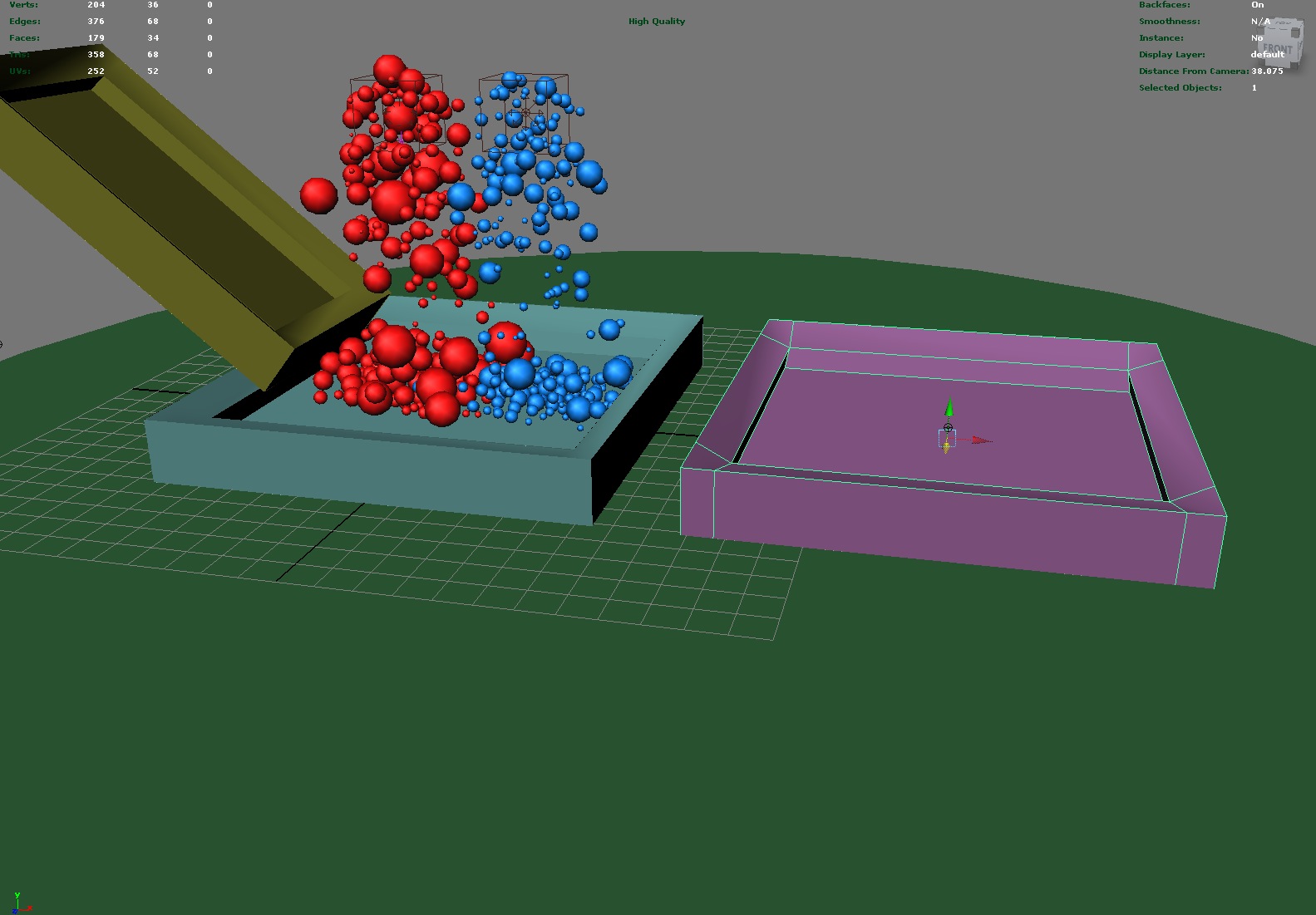
Under the collision attributes of the particles I enabled collide and set the width scale to 1 so the balls collide with each other. This value or one is the radius value of the particle, if less than this they radius will overlap and if larger then the will not touch. I varied the radius of the two particles to 0.4 and 0.5 with the randomise attribute set to 0.2 and 0.3 to make it visually more interesting with different sizes. I also adjusted the ramp in Radius Scale and set to Randomise ID on the radius scale input, this pick a number along the graph and applies the radius.
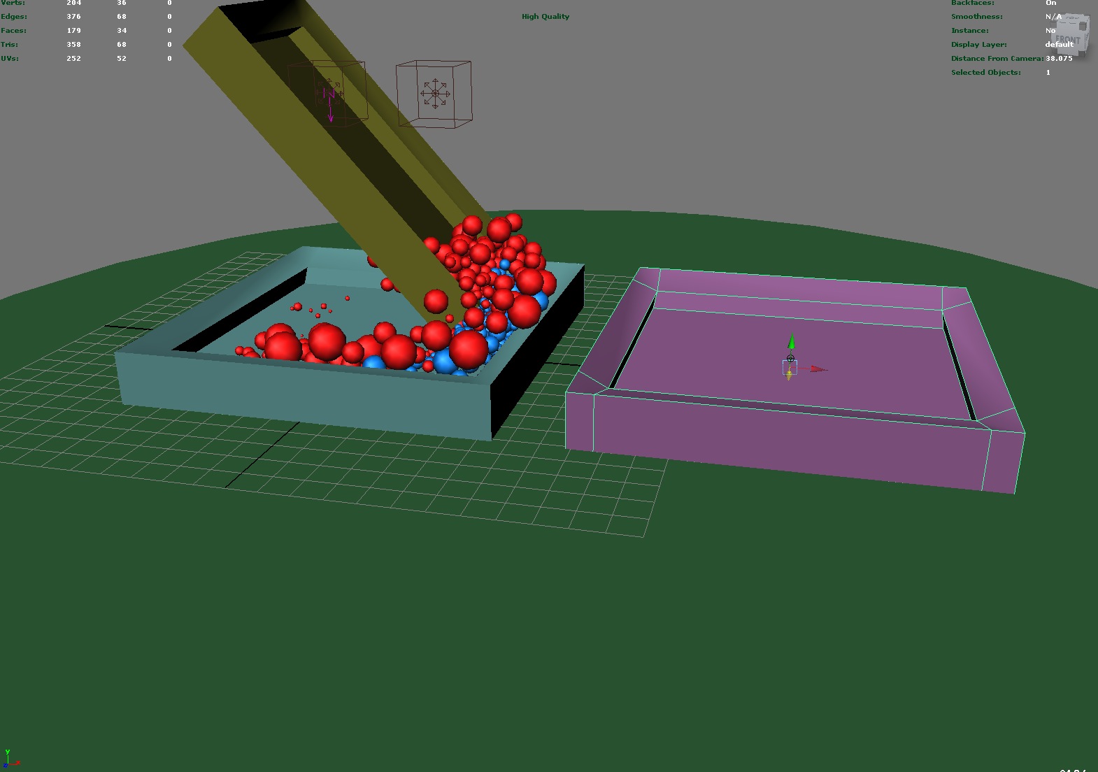
The trays have been made passive colliders and have an nRigid node. On the landing tray it has some bounce, a little bit of friction and stickiness. The pick up tray has friction set to 0.4, stickness to 0.2 and no bounce. The landing tray has some bounce of 0.2, friction to 0.1 and stickiness to 0.7.
On the particleShape node under Dynamic Attributes I left the Ignore Solver Wind and Gravity un-ticked and did not adjust the drag. The drag is like conserve on the standard particles where the 1 keeps the velocity constant. If the field are ticked then it is possible to add fields separately.
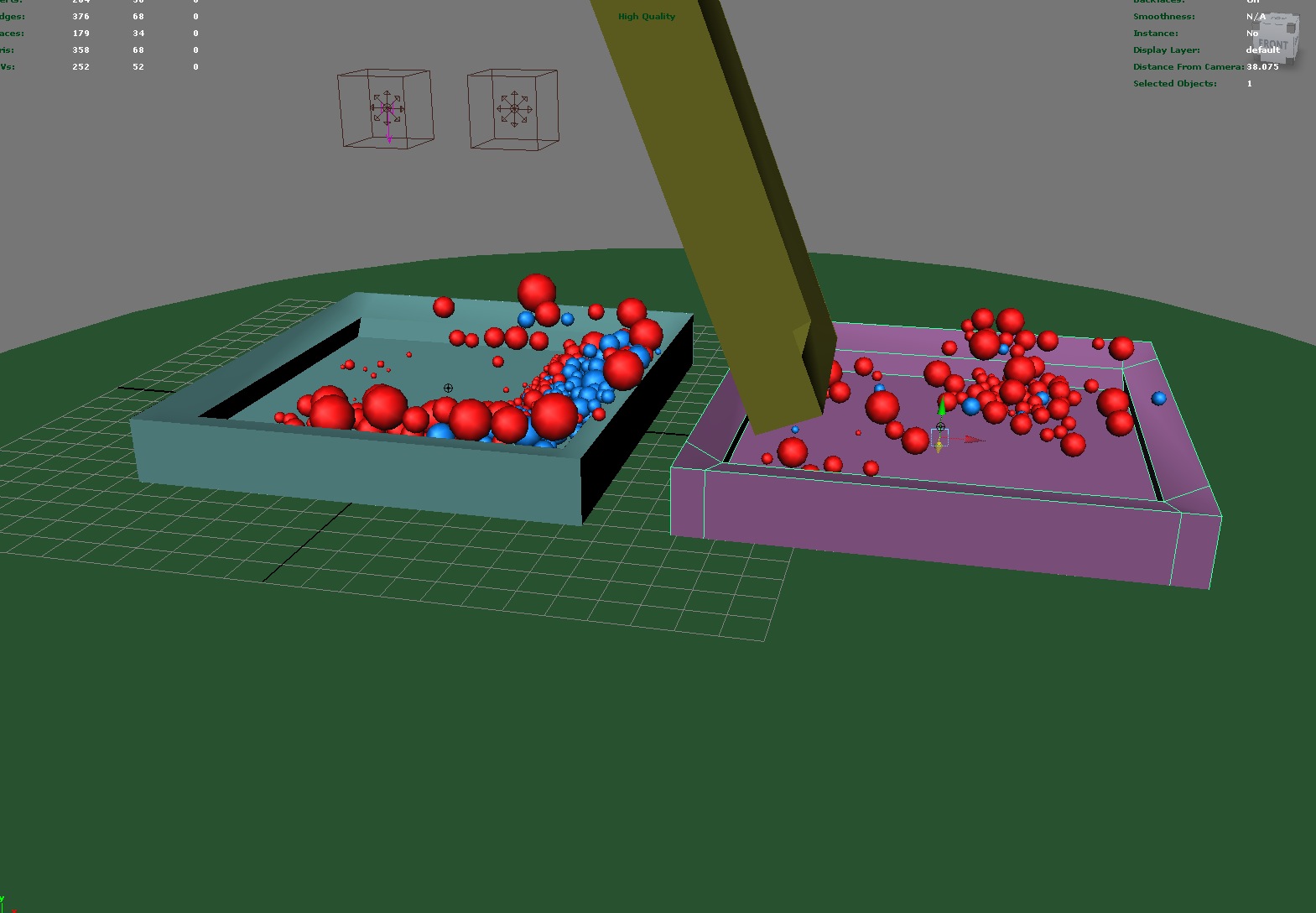
It is possible to start the simulation with the balls already in the ball pit by setting an initial state under nSolver.
The problem that is unresolved is how to have the balls the stick to the sides and on top of the sides fall into the tray. Still working on the rate at which the 200 balls are emitted so I can have more control over when it happens. The other thing is how do I control how many balls get picked up and how many are left behind.

WEEK FOUR Challenge
Waterfalls: Goal Weights and Goal Weights on Deformed Geo


Some References for the waterfall from Getty Images

geometry texture set up with a texture deformer
The geometry has been set up with lots of spans/resolution on the polygon plane due to altering the shape. Deforming the geometry with the texture deformer based is based on the texture mapped into the deformer’s texture attribute. It has been set up with an Ocean Texture and adjusting the
– turbulence
– wave height
– time expression =frame/20 into the field next to time to change the texture over time
– direction of the water movement is adjusted under Wind UV attributes, not sure how this is looking at the moment and will come back to it
– strength attribute for the height of the waves, 10 and the Offset attribute is set inversely, -10
-

- goal weight under goal weights and objects set to 1
-

- goal weight under goal weights and objects set to 0.5
It is the pivot point of the geometry that gets attached to the particle and they are in the same position. The particles are emitting directly from the geometry, there is no geometry linked to the particles with the Particle Instancer so I will leave the pivot point where it was positioned when the geometry was created. It is not like when we considered the pivot point of the cars that were instanced to particles that were then moving along the ground plane. I will see how this works with the water/particles moving directly across the geometry.
The emitter has been created to emit from object and under particles they are goal to the surface as a surface emitter. For now the Goal Weight has been set to one, with the particles sticking to the surface. When the Goal Weight is zero, the goal doesn’t have effect, this attribute can be animated. From what I can see at 1 the particles are moving with the deformed texture.
The particles are lining up in straight lines along the UV’s. Each vertex is numbered and the particles line up in order, in order to make sure the whole surface is covered the geometry needs to be normalised. This is checked in the UV texture editor and the surface fits into the 0 to 1 grid.
-

- assigned particle attributes and expressions
-

- particles not emitting on the whole surface
-

- Need Parent UV attributed enabled and particles emitting on surface
Under the Per Particle Attributes not all attributes are listed include the goal U & V attributes, add these and the parentV and parentU attributes. The parent U and parent V attributes are the positions on the surface where the particle are born and it is related to the emitter. Add the following creation expression influencing where the particles are created, being executed when the particles start to come out.
particleShape1.goalU = parentU;
and particleShape1.goalV – parentV;
The Need Parent U/V attribute needs to be enabled when using surface emissions for Nurbs/poly surfaces and now the particles are scattered all over the surface.
Expression under Per Particle (Array) Attributes, the particles will stick to the surface. When I made this 0.5 then when the particles were emitted they did not stick to the surface, zero would mean there would be no influence when the particles are created.
goalPP = 1;
Creating a Runtime Expression to add or alter the particle’s behaviour on each frame, in the Expression Editor. The Runtime Before Dynamics Expression allows us to make changes to the particle before the dynamics of the scene are calculated, before Fields and Collisions are calculated. For Runtime After Dynamics the expression will be executed after the dynamics are calculated. The following expression has been set on the goalPP attribute and says when the particles reach a position more than 0.99 on the texture grid then the goalPP will be zero, meaning there is no influence on the particle sticking to the surface. As the notes say the particles are not moving yet so I cannot see this in action.
if (goalU>0.99)
{
goalPP = 0;
}

if (water_particleShape1.goalU>0.99) { water_particleShape1.goalPP = 0; }
The +0.01 in the expression takes the position of the particle and moves it 0.01 maya units every frame in the U direction. It was not working at first and I needed to add the water_particleShape1 to the expression. Now I can see the direction the particles are moving and what they are doing when they leave the surface.
Random speed attributes added though the Expression Editor, made a new attribute and cannot remember about Scalar or Per particle (array), left it on Scalar, will see what happens.
Maya help files:
Scalar: Creates a per object attribute that you can set to a single value that applies to every particle in the object. A vector scalar is considered a single value with three numbers. If you select Scalar, you can specify Minimum,Maximum, and Default values for a Float or Integer attribute.
Per Particle (Array): Creates a per particle attribute. You can set this type of attribute to different values for each particle. If you select Per Particle (Array), you can also create a counterpart initial state attribute by turning on Add Initial State Attribute.
The randSpeed is now showing in the Expression Editor, the Creation Expression:
randSpeed = rand(0.01,0.02) and changed the Runtime expression from 0.01 to
water_particleShape1.goalU = water_particleShape1.goalU +randSpeed;
Going back to have another look at this and will make the the custom attribute with Per Particle (array) as it has not come up in the list of attributes , I seem to remember it did and I cannot find where the attribute is when I chose Scalar. That is working, it has come up in the Per Particle Attribute list and is at the bottom of the list of names in the Expression Editor.
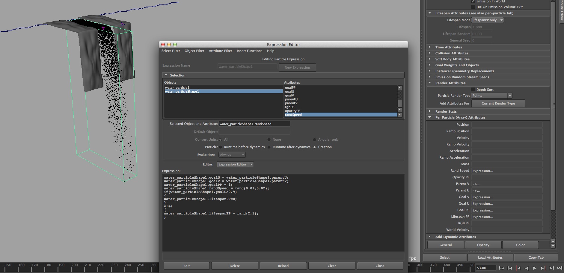
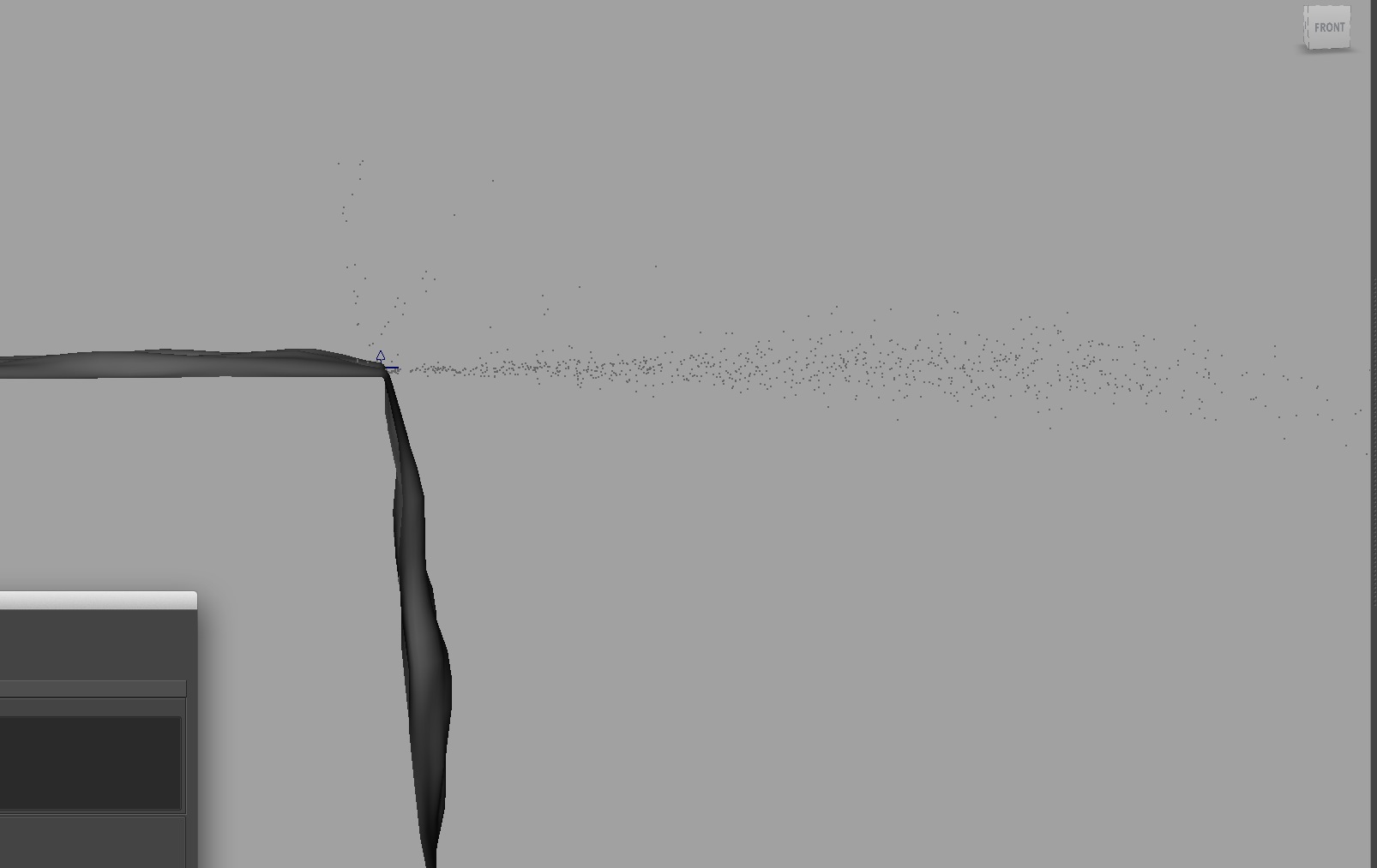
water_particleShape1.goalU= water_particleShape1.goalU + 0.01; or could be written as goalU =+0.01;

with gravity and drag field assigned using preset values
Maya Help Document
Gravity Field, the most commonly used field, it causes objects to move and accelerate in a given direction. You can limit its reach to create localized gravity fields. It simulates the Earth’s gravitational force.
Magnitude: sets the strength, the greater the magnitude, the faster the objects will accelerate in the direction of the gravitational force.
Attenuation: Sets how much the strength of the field diminishes as distance to the affected object increases. The rate of change is exponential with distance; the Attenuation is the exponent. If you set Attenuation to 0, the force remains constant over distance.
Falloff Curve: Available when Use Max Distance is checked. When using a field to exert force, sometimes the object receiving the force may have trouble settling down after the force is exerted. Use this curve to modulate the force. For example, scale the field’s force so that it smoothly drops off to zero at the boundary defined by the Max Distance value. The curve is defined within the normalized distance; in other words, 0 to 1, where 0 corresponds to the field’s center and 1 corresponds to the Max Distance value. The value from the curve is a scaling factor to be applied to the force.
Drag Field slows the momentum over time of objects within its reach. A drag field exerts a friction or braking force on an object that’s animated with dynamic motion.
Speed Attenuation: Weakens the amount of drag when the speed of the particle is less than the Speed Attenuation value. This allows slow moving particles to not be affected much by the drag, while heavily damping still occurs with fast moving ones. Available in the Attribute Editor only.
The fields are created at origin and for these fields it does not make any difference, when I move the emitter the act the same. I have set the magnitude to 40, if it is too high then the particles that are running along the geometry start to be affected and I want the gravity to work when they leave the surface geometry. I think there is probably an expression that I can write in the magnitude field to only have the gravity field affect the particles after they leave the surface and still thinking about this. The trade off is finding the point between having the particles fall directly down and have them falling as they are going along the geometry and less of this and not so straight when coming off the edge. Leaving the attenuation at zero keeps the particles falling down, when it is at one the particles appear to have no gravity affecting them. The direction is -1 in Y.
In the drag field I have set the magnitude to 2 as larger values cause the particles to not move over the edge at all or very slowly and it does not look natural. I used 2 and with Attenuation turned off the particles are falling straight down and I prefer some spraying type behaviour to be happening and have set this to 2 for now. I have left the Speed Attenuation at zero.
I have not used the Max Distance attribute on the fields as this creates a radius of influence and if the attenuation is set to zero there is a hard boundary created. From what I can see the idea to use a Drag Field slowing the momentum over time is enough.
if(goalU>0.9) { lifespanPP=0; } else { lifespanPP = rand(4,5); }
Using lifespanPP we can create an expression to stop the particles being born at the very end of the geometry. On the position of the surface that is greater than 0.9 then no particles will be born and they have a random lifespan range between 4 and 5, when I make it 8 and 9 they live longer and the length of the water falling is longer. I have made it 2,3 and they life a little either side of the geometry.
I have a better understand about the scripting this time and I think it is a combination of the MEL scripting classes and some time to process the information.
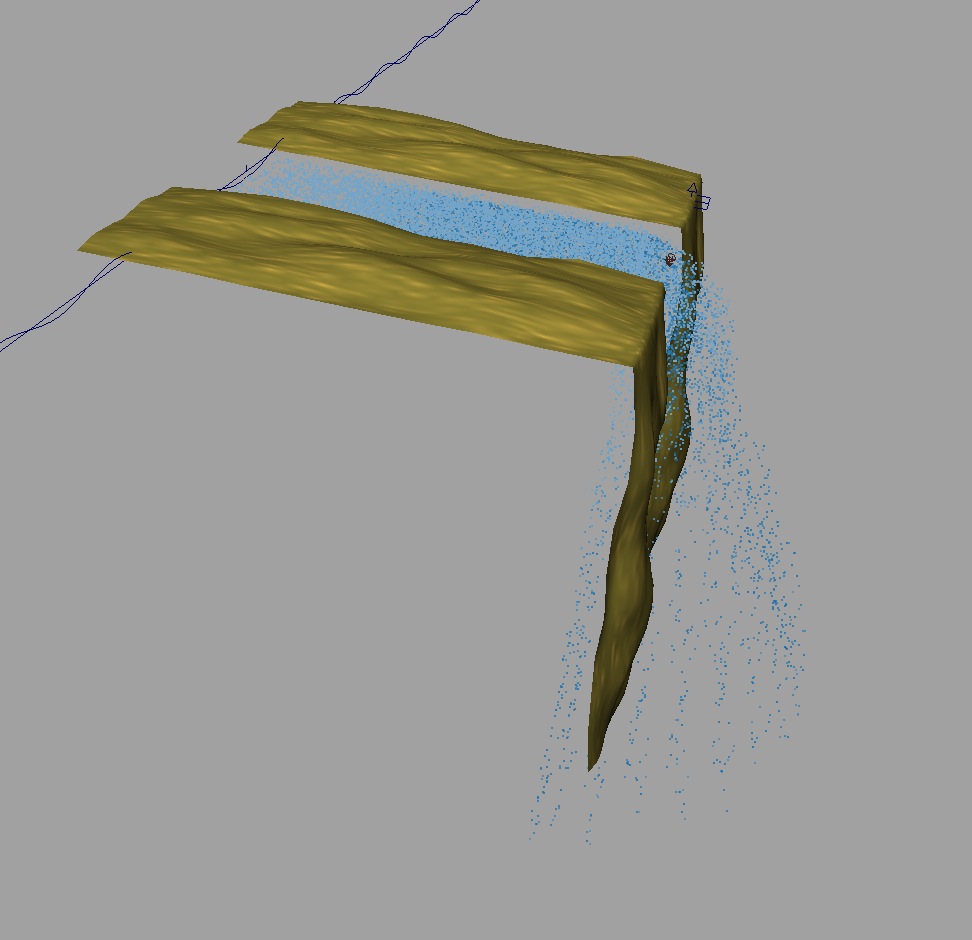
I have added ramp to the colour and opacity PP attribute and left the colourAccum off.
ColorAccum Adds the RGB components of overlapping particles. Also adds opacity values of overlapping particles. Generally, colors become brighter and more opaque as they overlap. To see the effect of Color Accum, you must add an opacity attribute to particles displayed asPoints. Valid for MultiPoint, MultiStreak, Points, andStreak render types. Maya Help Files
I have left the Max Count at -1, Sets a limit on the number of particles the emitted particle shape accepts from an emitter, which means they are will continue to be created. A number in this value controls how many are created.

showing where the multiStreaks are going above and below the geometry for the river bed and the falling motion could look more natural

multiStreaks settings
Other things to consider:
Over Samples where a value of 3 would calculate the position of the particles 3 times per frame.
Using a rig that controls the values from an expression.
WEEK TWO Challenge
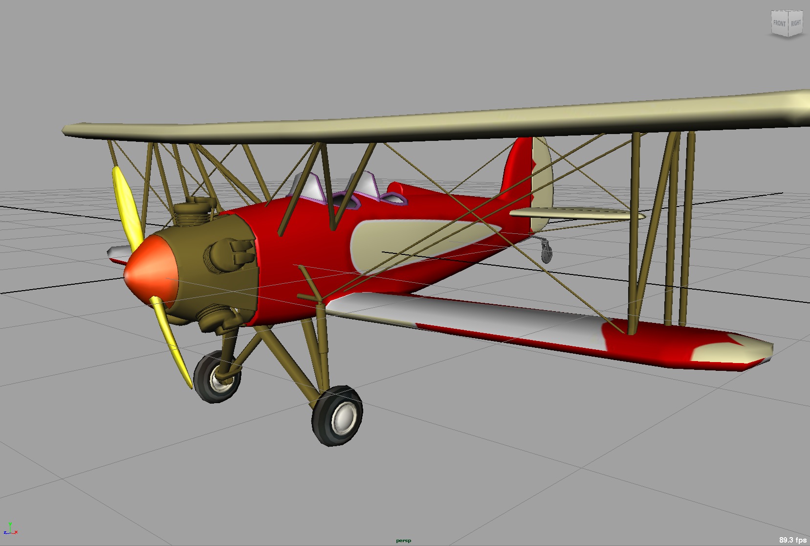
Use the Particle Instancer to create a squadron of planes flying through the air.
– 72 planes
– flying towards the camera over 100 frames
– each plane to have a unique motion such as orientation when it moves up/down in space, different speeds
– render the sequence with the supplied textures and own shaders which can be basic
– can include an Image Plane for the sky and it needs to match the camera angle
-

- with the plane geometry ungrouped and the propellor grouped
-

- grouping all the geometry and instanced this group to the particle
We learnt about the Particle Instancer which assigns instanced geometry, which is a copy, to particles so that it can inherit the motion of the particles.
– grouped the geometry with the the propellor animated in rotation z as a sub-group. Consider selecting all the geometry and then create the Instancer and will appear as individual items, an array
– freeze transformations and delete history
– centre pivot and geometry at origin
– created a volume emitter, cboxshape and scaled the length to spread the planes out across the sky
– group is instanced to the particle and a new node has been created and seen in the outliner
The propellor is rotating when I play the scene, yip, hee. When I animated the rotation on the propellor and cone seperately the pivot point needed to be changed so did it with them grouped and the group pivot point worked for the animation
– hide the original geometry
My camera view is the default X, Y, Z in perspective
– moved the emitter and rotated the original 90 in Y for the planes to point in the direction of the camera, still not flying in the right direction. Back to the drawing board. I rotated the original and redid the above and they are now pointing towards the camera.
– setting the max count to 75 and adjusting the rate to stager when the planes fly across the sky. When rate is too low, like 5 the 75 planes are not born when the 100 frames is reached. Made the rate (particles/sec) 20 and I like the look.
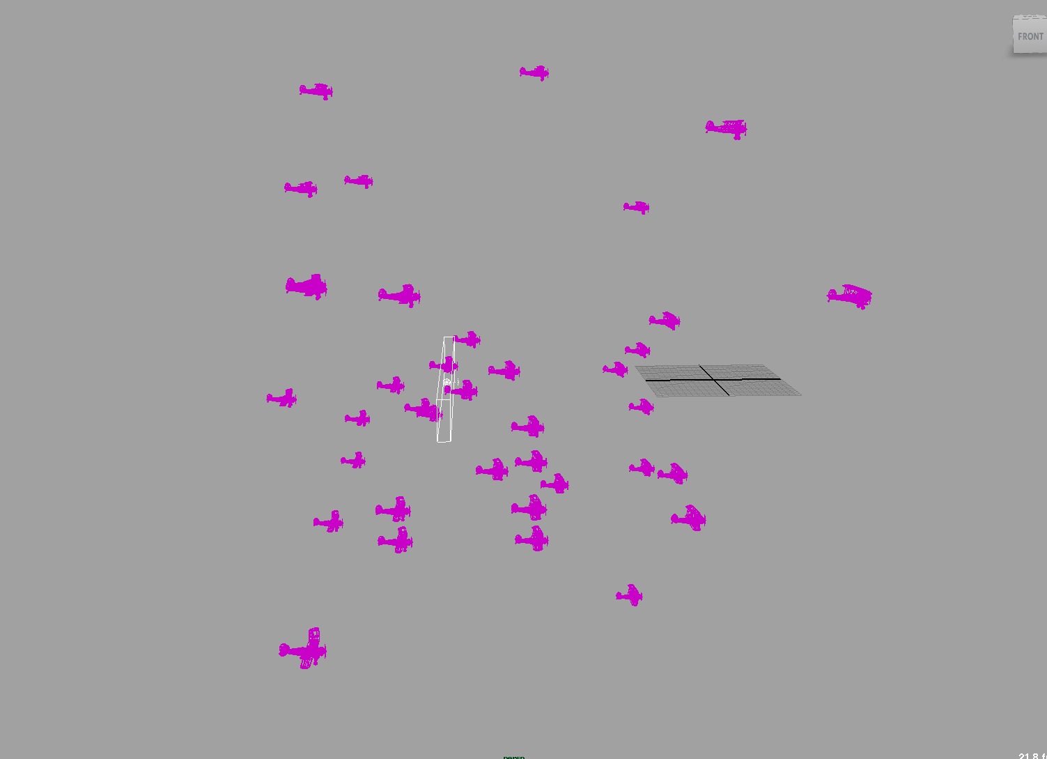
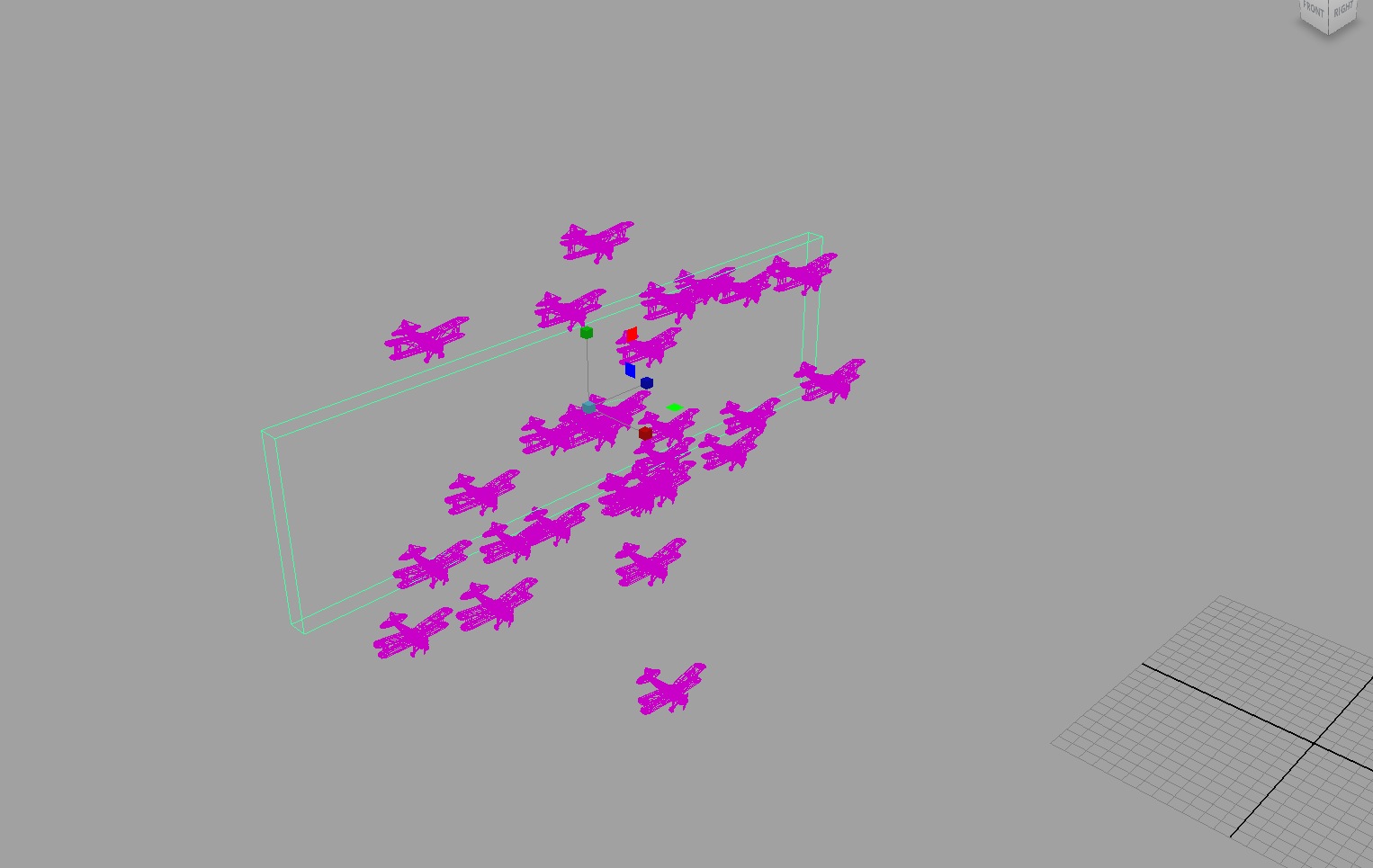
They are still to clumped together, have scaled the volume emitter in Y as well as Z and they look better spread out. Still not looking right, they need to fly across the screen and not be so clumped together. After looking directional attributes, and attributes on the particle I still think it would have something to do with the emitter. Looking back at the emitter attributes the away from centre or along axis is not helping, so not sure how to have them fly like they are going forward. Finally when I adjust the Directional Speed they are going in different directions with some control. It appears that the faster speed contributes to controlling them to move forward.
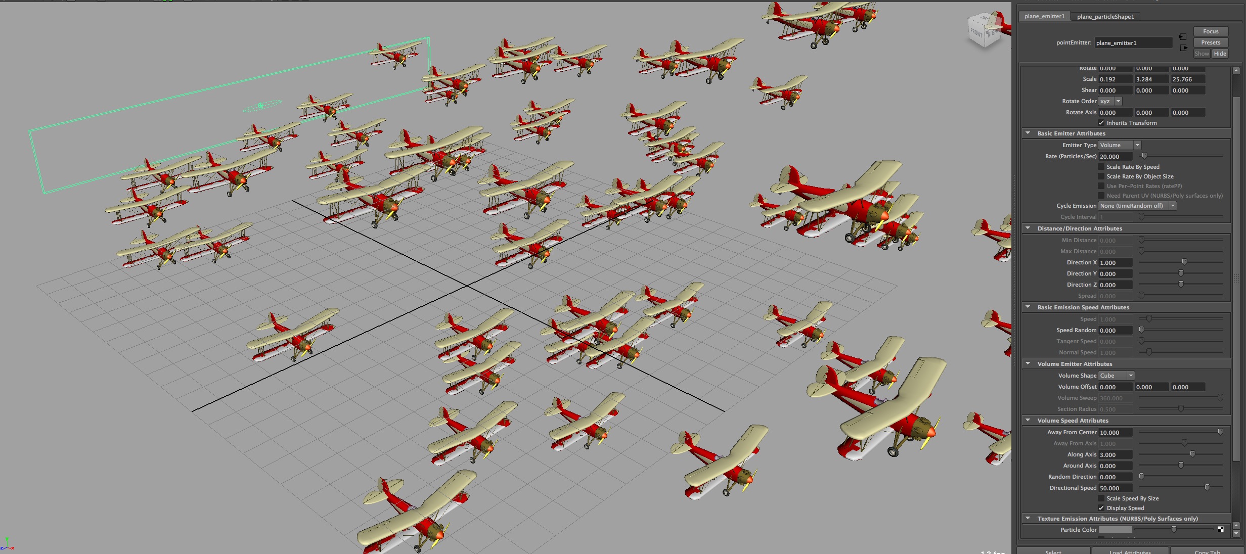
Changed the along axis to 5: Specifies the speed at which particles move along the central axis of all volumes. The central axis is defined as positive-Y for cube and sphere volumes.
The Away from Centre to 5: Specifies the speed at which particles move away from the center point of cube or sphere volumes
Directional Speed to 50: Adds speed in the direction specified by the Direction XYZ attributes of all volume emitters.
I have 75 planes flying over 100 frames in the direction of the camera, now to add some variety giving each plane some unique motion such as orientation when it moves up and down in space and the speeds. Changing the position, height and width of the volume emitter’s, Cube shape changes where the planes are emitted from, adding depth and width to the flight path as well as its starting point.
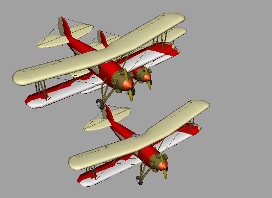
all the propellors are rotation the same
Now I would like to see how some fields work to introduce the variety in the motion. Initially thought about a Turbulence field and will start with an air field looking at the Wind, Wake, and Fan options.
In a later week we learnt about initial state under solvers, which would have the 72 planes already flying on the first frame or I could move the emitter off screen.
I love the colours and thanks for having the textures.
Reference:
WEEK ONE Challenge
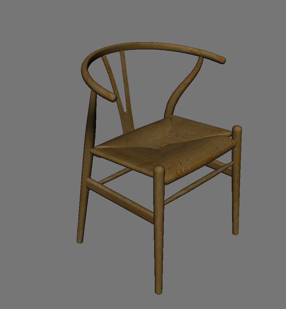
Make a chair out of particles and have it blow away with either a fan or in the breeze.
I set up the project with settings of 25 fpc, realtime, play every frame, set a larger frame range in the time slider and start at 1:00. Then scale the chair to real world scale, maya is in cm and scaled the model by 35 and using the wood veneer texture. The centre point needs to be at origin, modified the centre pivot for the chair then snapped to origin. Now the transforms have an offset so need to freeze transformations.
Creating a surface emitter, using the chair geo as the emitter so the particles emit from it, otherwise they emit from the vertex points. The emitter becomes the child of the chair and travels with it.
I needed to have the chair covered in particles and work out how to blow them away.


What I learnt doing this was to use the Rate (rate/sec) on the emitter to set the number of particles at 5000. The speed is set to 0 so they do not move away. Instead of using the time attributes to start the particles I could already have them covering the chair by setting the initial state under solvers. This was learn’t in later classes and meant I could cancel the ideas I had of turning the visibility off on the chair after the particles had covered them. My chair is invisible from the beginning and already covered in particles from frame one.
The texture is added to the particles on the emitter’s attributes under Texture Emission Attributes. The file is mapped in on a file node and inherit colour is ticket.
This is where I explored the used of different fields, their attributes and animating the values. I used a combination of air, turbulence and gravity to create different shapes with the particles moving from the chair. I animated the magnitude on the fields, adjusted the attenuation, the directions and animated the magnitude values. I decided to delete the gravity field and changed the airField to wind. There still needs to be more randomness in the look of the particles breaking up and could look more like they are being blown away by a fan or in a breeze.


Fields are localized or global forces that act on objects. You can simulate the motion of natural forces with dynamics fields.Fields have their own icons in a scene, so it’s easier to select them if you want to animate a field or change its attributes. These fields are included with Maya.
Stand-alone fields influence objects from a stationary or moving position in the workspace. It’s not owned by geometry.
Object Field are owned by an object and exert influence from the object. You can add fields to polygons, Nurbs curves or surfaces, particle objects, lattices or curves on the surface.
Volume Fields you can select a volume to define the region in space in which particles are affected.
The following fields are included with Maya:
- Air An air field simulates the effects of moving air. The objects you connect to the air field accelerate or decelerate so their velocities match that of the air as the animation plays. A “push” type of field, it comes with presets for Wind, Wake, and Fan.
- Drag a field that slows the momentum over time of objects within its reach. A drag field exerts a friction or braking force on an object that’s animated with dynamic motion.
- Gravity The most commonly used field, it causes objects to move and accelerate in a given direction. You can limit its reach to create localized gravity fields. It simulates the Earth’s gravitational force.
- Newton Similar to gravity, but operates in a spherical manner. A newton field pulls object towards it. Objects are attracted to Newton fields more strongly depending on their mass and their distance from the Newton field.
- Radial A radial field pushes objects away or pulls them toward itself, like a magnet. Like the Newton field, but it doesn’t take mass into account. It can be set to diminish with distance, as with the Gravity and Air fields, and it can be set to push or pull.
- Turbulence Makes the object’s motion or deformations more random. Turbulence is usually applied to soft bodies or particles to create the impression of wind or waves.
- Uniform A field that pushes objects in a specified direction. Like the Gravity field, but without the progressive acceleration that Gravity includes.
- Vortex A kind of rotating gravity, the Vortex field pulls objects in a spiraling motion that’s centered on the field’s icon. Often used to create galaxies, whirlpools, or tornados with particle systems.
- Volume Axis A complex field that lets you specify a volume shape (cube, sphere, cylinder, cone, or torus) and then create effects that work within the shape. You can use the Volume axis field to create effects such as particles flowing around obstacles ,solar flares, mushroom clouds, explosions, tornadoes, and rocket exhaust.
OTHER REFERENCES
YOUTUBE
Falling Stuff – Rigid Body Tests
Contours of Vorticity of Vertical Axis Wind Turbine in ANSYS FLUENT – Vorticity
